Part 3: Model-Level Interventions (In-Processing)

Context

In-processing interventions embed fairness directly into model training, addressing bias that persists despite data-level fixes.

This Part equips you with algorithms that optimize for both accuracy and fairness simultaneously. You'll learn to reshape how models learn rather than just modifying inputs or outputs. Too many practitioners treat fairness as an afterthought rather than a core optimization criterion.

Constraint-based methods enforce fairness during training. A hiring algorithm might include constraints ensuring similar acceptance rates across demographic groups, preventing it from learning historical biases while still capturing legitimate predictive signals. These constraints reshape the solution space, guiding models toward regions where fairness and performance coexist.

Adversarial approaches leverage competing objectives to neutralize bias. By pitting a predictor against a discriminator that tries to infer protected attributes, models learn representations that preserve predictive power while becoming "blind" to sensitive features. This mirrors how GANs work, but with fairness as the goal.

These interventions transform how you build models—from loss function formulation through hyperparameter selection to evaluation strategies. Techniques range from simple regularization terms to sophisticated multi-objective optimization frameworks that navigate fairness-performance trade-offs.

The In-Processing Fairness Toolkit you'll develop in Unit 5 represents the third component of the Fairness Intervention Playbook. This tool will help you select and implement appropriate algorithmic interventions for different model architectures, ensuring fairness becomes intrinsic to how your models learn.

Learning Objectives

By the end of this Part, you will be able to:

Implement fairness constraints within model optimization objectives. You will formulate mathematical constraints that enforce group fairness criteria during training, enabling models that natively satisfy fairness definitions rather than requiring post-hoc corrections.
Design adversarial debiasing approaches for neural networks. You will create model architectures where adversarial components remove protected information from learned representations, preventing discrimination while preserving useful predictive patterns.
Apply regularization techniques that promote fair learning. You will integrate fairness-specific regularization terms into objective functions, guiding models away from discriminatory solutions through penalization rather than hard constraints.
Develop multi-objective optimization strategies for balancing fairness and performance. You will implement training procedures that navigate the Pareto frontier between competing objectives, creating models that achieve optimal trade-offs rather than sacrificing either fairness or accuracy.
Adapt in-processing techniques to different model architectures. You will modify fairness interventions to work across diverse model types from linear classifiers to deep networks, ensuring fairness remains achievable regardless of your modeling approach.

Units

Unit 1

Unit 1: Fairness Objectives and Constraints

1. Conceptual Foundation and Relevance

Guiding Questions

Question 1: How can abstract fairness definitions be translated into concrete optimization objectives and constraints that algorithms can directly optimize during training?
Question 2: What are the mathematical and computational implications of incorporating fairness constraints into model optimization, and how do these affect model performance?

Conceptual Context

When developing machine learning models that make consequential decisions, fairness cannot be an afterthought. While pre-processing approaches modify training data before model development, in-processing techniques directly integrate fairness into the learning algorithm itself. This integration creates models that are inherently fair by design rather than attempting to correct unfairness after training.

Constraints and objectives form the mathematical core of machine learning optimization. Standard algorithms typically optimize a single objective (such as accuracy or log-likelihood) without explicit fairness considerations. By reformulating these optimization problems to include fairness definitions as explicit constraints or additional objectives, you can develop models that balance traditional performance metrics with fairness requirements during the training process itself.

This approach is particularly valuable because it addresses fairness directly in the model's decision boundary rather than through indirect data modifications. As Dwork et al. (2012) noted, "Solutions that rely exclusively on data pre-processing cannot guarantee fair decisions if the underlying algorithm can still construct biased decision boundaries." In contrast, in-processing approaches provide mathematical guarantees about the fairness properties of the resulting model.

This Unit establishes the foundation for all subsequent in-processing techniques by showing how fairness definitions can be translated into the language of mathematical optimization. You'll learn how to formulate constrained optimization problems that enforce fairness requirements while maintaining predictive performance. This understanding will directly inform the In-Processing Fairness Toolkit you'll develop in Unit 5, enabling you to select and implement appropriate in-processing techniques for specific fairness challenges.

2. Key Concepts

Translating Fairness Definitions to Mathematical Constraints

Fairness definitions provide conceptual criteria for equitable treatment, but to incorporate them into model training, you must translate these definitions into precise mathematical formulations that algorithms can optimize. This translation process is fundamental for in-processing techniques because it transforms abstract fairness goals into concrete computational objectives.

Different fairness definitions require different mathematical formulations. For example, demographic parity can be expressed as equality constraints on prediction rates across groups, while equalized odds requires conditional constraints that consider both predictions and ground truth labels.

This concept intersects with optimization theory by extending standard machine learning objectives to incorporate fairness. It connects to algorithmic implementation by requiring modifications to training procedures that can handle these additional constraints.

Zafar et al. (2017) pioneered this approach by showing how fairness constraints could be incorporated into logistic regression through convex relaxations. For demographic parity, they formulated a constraint that equalizes the mean prediction across protected groups:

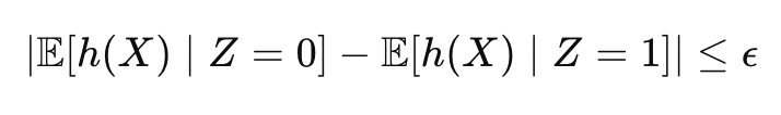
Where h(X) is the model's prediction, Z is the protected attribute, and ε is a small tolerance. This constraint ensures that the average prediction for different groups differs by no more than ε, directly enforcing the demographic parity criterion during training.

For the In-Processing Fairness Toolkit you'll develop, understanding these translations is essential for implementing fairness constraints across different model types and fairness definitions. This knowledge enables you to select appropriate constraint formulations for specific fairness requirements and model architectures.

Constrained Optimization Approaches

Once fairness definitions are translated into mathematical constraints, you must integrate these constraints into the learning process through constrained optimization techniques. This integration is essential for in-processing because it determines how the algorithm will navigate the trade-off between its original objective and the fairness constraints.

Standard machine learning models typically minimize an unconstrained loss function: min₍θ₎ L(θ)

Where L(θ) represents the loss function (e.g., cross-entropy loss) and θ represents the model parameters. To incorporate fairness, this problem is reformulated with constraints:

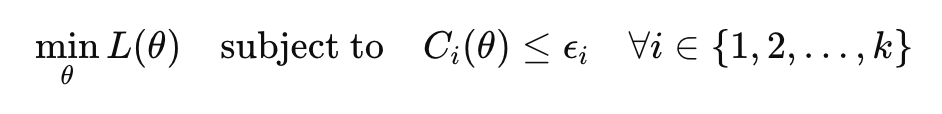
Where Cᵢ(θ) represents fairness constraint functions and εᵢ represents tolerance levels for each constraint.

This concept interacts with fairness definitions by determining how strictly different fairness criteria will be enforced. It connects to practical implementation by influencing both algorithm selection and computational requirements, as constrained optimization is generally more complex than unconstrained approaches.

Agarwal et al. (2018) demonstrated how constrained optimization for fairness could be implemented through a reduction approach that converts constrained problems into a sequence of unconstrained ones. Their method enables the application of fairness constraints to any model class with standard training procedures, making constrained fairness more broadly applicable.

For the In-Processing Fairness Toolkit, understanding these optimization approaches is crucial for implementing fairness constraints across different model architectures. This knowledge helps you select appropriate algorithms based on the mathematical properties of your constraints and the computational resources available for training.

Lagrangian Methods and Duality

Lagrangian methods provide a powerful framework for solving constrained optimization problems by incorporating constraints into the objective function through Lagrange multipliers. This approach is particularly valuable for fairness because it transforms hard constraints into soft penalties that can be more easily optimized.

The Lagrangian formulation of a constrained fairness problem takes the form:

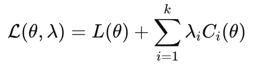
Where λᵢ are Lagrange multipliers that control the importance of each constraint. This formulation allows algorithms to balance the original objective against fairness requirements through appropriate tuning of the multipliers.

This concept connects to constraint enforcement by determining how strictly fairness requirements are maintained. It relates to regularization approaches by showing how constraints can be reformulated as penalties in the objective function.

Cotter et al. (2019) extended Lagrangian methods for fairness by developing a proxy-Lagrangian formulation that handles non-differentiable constraints more effectively. Their approach enables training with multiple fairness constraints simultaneously, allowing for more comprehensive fairness guarantees.

For the In-Processing Fairness Toolkit, understanding Lagrangian methods is essential for implementing fairness constraints in ways that balance enforcement with optimization stability. This knowledge enables you to transform strict fairness constraints into more flexible formulations that can be optimized efficiently while still providing strong fairness guarantees.

Feasibility and Trade-offs

Incorporating fairness constraints into optimization creates fundamental trade-offs between competing objectives and raises important questions about constraint feasibility. Understanding these trade-offs is critical because it determines what combinations of fairness and performance are achievable in practice.

The feasible region for a constrained optimization problem is the set of all parameter values that satisfy all constraints. When fairness constraints are too strict or conflict with the data structure, this region may be very small or even empty, making the problem infeasible. Even when feasible solutions exist, fairness constraints typically reduce the model's performance on traditional metrics.

This concept intersects with impossibility theorems by illustrating the practical implications of mathematical limitations. It connects to implementation decisions by influencing how strictly fairness constraints should be enforced in different contexts.

Menon and Williamson (2018) analyzed these trade-offs mathematically, showing how different fairness constraints affect the achievable accuracy. Their work provides theoretical bounds on performance losses when enforcing fairness constraints, helping practitioners understand the costs of different fairness requirements.

For the In-Processing Fairness Toolkit, understanding these trade-offs is essential for setting appropriate fairness constraints and communicating their implications to stakeholders. This knowledge enables you to navigate the fairness-performance frontier effectively, finding solutions that provide meaningful fairness guarantees while maintaining acceptable performance for your application.

Domain Modeling Perspective

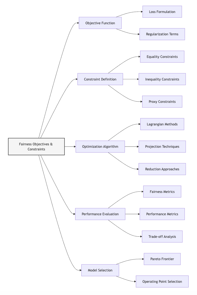
From a domain modeling perspective, fairness objectives and constraints map to specific components of ML systems:

Objective Function: Fairness considerations can be incorporated as additional terms in what the model optimizes.
Constraint Definition: Fairness criteria can be enforced as boundaries on acceptable model behavior.
Optimization Algorithm: The solution approach must be adapted to handle fairness constraints efficiently.
Performance Evaluation: Both traditional metrics and fairness criteria must be considered when assessing models.
Model Selection: Trade-offs between fairness and performance influence which model is ultimately deployed.

This domain mapping helps you understand how fairness constraints affect different aspects of model development rather than viewing them as isolated modifications. The In-Processing Fairness Toolkit will leverage this mapping to guide appropriate constraint implementations based on which components can be modified in your specific context.

Conceptual Clarification

To clarify these abstract optimization concepts, consider the following analogies:

Translating fairness definitions to constraints is similar to converting building codes into architectural specifications. Just as architects must translate requirements like "accessible to wheelchair users" into concrete measurements (door widths, ramp angles), machine learning engineers must translate fairness definitions like "demographic parity" into precise mathematical expressions that constrain the model's behavior. Both translations convert abstract principles into specific, measurable criteria that can be verified and enforced during construction/training.
Constrained optimization for fairness resembles navigating with route restrictions in GPS navigation. A standard navigation system might simply minimize travel time (like a model minimizing error), but adding constraints such as "avoid highways" or "avoid toll roads" is similar to adding fairness constraints. These constraints may lead to a longer route (reduced model performance) but ensure the journey satisfies important requirements. Just as the navigation system must find the fastest route that respects all restrictions, constrained optimization finds the best-performing model that satisfies all fairness constraints.
The feasibility-performance trade-off in fairness is analogous to budgeting with multiple financial goals. Imagine trying to simultaneously save for retirement, a home down payment, and an emergency fund with a limited income. Allocating more to one goal necessarily reduces what's available for others. Similarly, enforcing stricter fairness constraints typically reduces resources available for optimizing performance. In both cases, you must decide which goals are non-negotiable (hard constraints) versus aspirational (soft constraints) and find a balance that best satisfies your priorities given the resources available.

Intersectionality Consideration

Traditional fairness constraints often address protected attributes independently, potentially missing unique fairness concerns at intersections of multiple identities. As demonstrated by Kearns et al. (2018) in their work on subgroup fairness, models that satisfy fairness constraints for individual protected attributes may still discriminate against specific intersectional subgroups.

For example, a lending algorithm might achieve demographic parity across both gender and race categories independently, while still discriminating against specific intersections like women of a particular racial background. Standard constraint formulations would miss these intersectional disparities.

Implementing intersectional fairness through constraints requires:

Multi-attribute constraint formulations that consider all relevant demographic combinations.
Rich constraint specifications that can express complex fairness requirements across overlapping groups.
Computational approaches that handle the exponential growth in constraints as the number of protected attributes increases.

Foulds et al. (2020) addressed this challenge by developing an intersectional fairness framework that efficiently enforces fairness across exponentially many subgroups through statistical aggregation. Their approach provides stronger guarantees for intersectional fairness while maintaining computational tractability.

For the In-Processing Fairness Toolkit, addressing intersectionality requires constraint formulations that explicitly consider interactions between protected attributes. This might involve:

Separate constraints for important intersectional subgroups.
Hierarchical constraint structures that enforce fairness at multiple levels of granularity.
Statistical techniques that efficiently handle the combinatorial explosion of subgroups.

By incorporating these intersectional considerations, the framework will ensure that fairness constraints protect all demographic subgroups, not just those defined by single attributes.

3. Practical Considerations

Implementation Framework

To effectively translate fairness definitions into practical optimization constraints, follow this structured methodology:

Constraint Formulation:
Select appropriate mathematical expressions based on your fairness definition (demographic parity, equalized odds, etc.).
Determine whether to use equality constraints (C(θ) = 0) or inequality constraints (C(θ) ≤ ε).
Consider proxy constraints that approximate complex fairness criteria with more tractable expressions.
Document the mathematical formulation and its relationship to the original fairness definition.
Optimization Integration:
Select an appropriate constrained optimization algorithm based on constraint properties (convexity, differentiability, etc.).
Implement Lagrangian formulations that incorporate constraints into the objective function.
Develop efficient projection techniques for maintaining constraint feasibility during training.
Establish monitoring approaches for tracking constraint satisfaction throughout optimization.
Feasibility Analysis:
Verify that fairness constraints can be satisfied given the data distribution.
Identify potential conflicts between multiple fairness constraints.
Determine appropriate tolerance levels (ε) that balance strict fairness with achievable solutions.
Document feasibility findings to inform constraint adjustments if necessary.

These methodologies integrate with standard ML workflows by extending existing optimization procedures to handle fairness constraints. While they add complexity to model training, they enable direct enforcement of fairness properties that may be difficult to achieve through pre-processing alone.

Implementation Challenges

When implementing fairness constraints, practitioners commonly face these challenges:

Optimization Difficulties: Fairness constraints can create non-convex optimization landscapes that are harder to navigate. Address this by:
Starting with simpler constraint formulations and gradually increasing complexity.
Using advanced optimization techniques like alternating direction method of multipliers (ADMM).
Implementing warm-start approaches that begin from unconstrained solutions.
Monitoring convergence behavior and adjusting optimization parameters accordingly.
Constraint-Performance Trade-offs: Strict fairness constraints often reduce model performance on standard metrics. Address this by:
Analyzing the Pareto frontier to understand available trade-offs.
Implementing adjustable constraint formulations that can be tuned based on application requirements.
Developing multiple models with different constraint settings to provide options for stakeholders.
Creating clear visualizations that communicate trade-offs to non-technical decision-makers.

Successfully implementing fairness constraints requires computational resources for more complex optimization, expertise in mathematical programming and fairness definitions, and organizational willingness to potentially sacrifice some performance for improved fairness. The specific technical requirements will vary based on the model type and fairness criteria being enforced.

Evaluation Approach

To assess whether your fairness constraints are working effectively, implement these evaluation strategies:

Constraint Satisfaction Verification:
Calculate constraint violations on both training and validation data.
Monitor constraint satisfaction throughout training to identify potential instabilities.
Verify that constraints remain satisfied when the model is applied to new data.
Document constraint violations and their magnitudes to inform potential adjustments.
Performance Impact Assessment:
Quantify performance differences between constrained and unconstrained models.
Analyze which performance metrics are most affected by fairness constraints.
Determine whether performance impacts are acceptable given application requirements.
Identify specific subgroups or data regions where performance changes are most significant.

These evaluation approaches should be integrated with your organization's broader model assessment framework, providing a comprehensive understanding of both fairness properties and traditional performance metrics.

4. Case Study: Loan Approval System

Scenario Context

A financial institution is developing a machine learning model to predict default risk for loan applications. The model will be used to automate preliminary approval decisions, with higher-risk applications receiving additional manual review. The dataset includes financial history, current income and assets, loan amounts, and repayment history for past customers. Protected attributes like gender, age, and race are available for fairness analysis but should not directly influence decisions.

Initial unconstrained models showed concerning disparities: the approval rate for applicants from minority racial groups was 15% lower than for the majority group, even when controlling for relevant financial factors. The data science team must address this disparity while maintaining the model's ability to accurately predict default risk.

Key stakeholders include the bank's risk management team concerned with financial performance, compliance officers responsible for ensuring regulatory adherence, customers from diverse backgrounds seeking fair evaluation, and executives balancing business goals with ethical considerations. The fairness implications are significant given the potential impact on financial access and opportunity.

Problem Analysis

Applying the concepts from this Unit to the loan approval scenario:

Fairness Definition Translation: The team decided to enforce demographic parity for preliminary approvals, requiring similar approval rates across demographic groups. This definition translates to a constraint on the difference in mean predictions between protected groups:

Where h(X) is the model's prediction (approval probability), Z is the protected attribute, and ε is a small tolerance that allows for minor disparities due to legitimate differences in qualification.

Constraint Implementation: The team initially attempted to implement strict equality constraints (ε = 0), but found this infeasible given the genuine correlations between default risk factors and protected attributes in their historical data. They then explored inequality constraints with varying tolerance levels, finding that ε = 0.05 (allowing up to 5% difference in approval rates) provided a reasonable balance between fairness and feasibility.
Optimization Approach: For their logistic regression model, they implemented the constraint using a Lagrangian formulation:

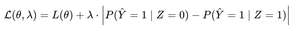
This formulation allowed them to adjust the Lagrange multiplier (λ) to control the trade-off between prediction accuracy and fairness.

Intersectional Considerations: Initial implementations focused only on racial disparities, but further analysis revealed unique challenges for specific intersectional groups, particularly young applicants from minority backgrounds with limited credit history. To address this, they extended their constraint formulation to include key intersectional categories, ensuring fairness across both individual attributes and their important combinations.

From a feasibility perspective, the team discovered that strict demographic parity (ε = 0) would reduce the model's default prediction accuracy by approximately 8%, while the relaxed constraint (ε = 0.05) reduced accuracy by only 3%. This analysis helped stakeholders understand the concrete trade-offs involved in different fairness requirements.

Solution Implementation

To address the fairness challenges through constrained optimization, the team implemented a comprehensive approach:

For Constraint Formulation, they:
Developed mathematical expressions for demographic parity that could be efficiently computed during training.
Created relaxed inequality constraints with adjustable tolerance parameters.
Extended the constraints to address key intersectional categories identified during data analysis.
Documented the relationship between their mathematical constraints and the fairness requirements.
For Optimization Integration, they:
Implemented a projected gradient approach for their logistic regression model.
Developed Lagrangian formulations that incorporated fairness constraints into the objective function.
Created an ADMM implementation for handling multiple constraints simultaneously.
Established monitoring procedures to track constraint satisfaction during training.
For Feasibility Analysis, they:
Analyzed the Pareto frontier to understand available trade-offs between fairness and default prediction.
Developed multiple models with different constraint settings (ε values ranging from 0.01 to 0.10).
Created visualizations showing both performance metrics and fairness properties for different constraint configurations.
Documented the achievable combinations of fairness and performance to inform stakeholder decisions.

Throughout implementation, they maintained explicit focus on intersectional effects, ensuring that fairness constraints protected all demographic subgroups rather than just addressing aggregate disparities.

Outcomes and Lessons

The constrained optimization approach yielded several key results:

The final model with ε = 0.05 reduced the approval rate disparity from 15% to 4.8%, while limiting the decrease in overall default prediction accuracy to 3%.
The intersectional constraints successfully addressed unique challenges for young minority applicants, reducing previously undetected disparities in this subgroup.
The constraint formulation provided mathematical guarantees about maximum fairness disparities, creating more transparent and defensible model properties compared to ad hoc adjustments.

The team faced several challenges during implementation, including optimization difficulties with multiple constraints and communication challenges when explaining trade-offs to stakeholders. They found that visualizing the Pareto frontier of fairness-performance combinations was particularly effective for facilitating informed decisions about constraint settings.

Key generalizable lessons included:

The importance of relaxed constraints with appropriate tolerance levels rather than strict equality constraints, which are often infeasible in real-world scenarios.
The value of training multiple models with different constraint settings to understand available trade-offs rather than committing to a single fairness-performance balance prematurely.
The necessity of explicitly addressing intersectional fairness through additional constraints rather than assuming protection of individual attributes will extend to their intersections.

These insights directly inform the In-Processing Fairness Toolkit in Unit 5, demonstrating how theoretical constraint formulations translate into practical fairness improvements in high-stakes applications.

5. Frequently Asked Questions

FAQ 1: Mathematical Formulation Choices

Q: How do I choose between equality constraints, inequality constraints, and Lagrangian formulations when implementing fairness in my model?
A: The choice depends on your fairness requirements, optimization capabilities, and application context. Equality constraints (C(θ) = 0) provide the strongest fairness guarantees by requiring exact satisfaction of fairness criteria, but they're often infeasible or lead to significant performance degradation in real-world scenarios with underlying data disparities. Inequality constraints (C(θ) ≤ ε) offer more flexibility by allowing small fairness violations up to a tolerance threshold, making them more practical while still providing meaningful guarantees. Lagrangian formulations transform constraints into penalty terms in the objective function, offering the most flexibility by allowing you to control the fairness-performance trade-off through multiplier tuning.

Generally, start with Lagrangian formulations during exploratory analysis to understand potential trade-offs. If you need formal guarantees, transition to inequality constraints with appropriate tolerance levels based on your exploration. Reserve equality constraints for scenarios where perfect fairness is absolutely required and feasibility analysis confirms they can be satisfied. Your choice should also consider computational factors: equality constraints often create harder optimization problems, while Lagrangian approaches can work with standard optimization algorithms. Finally, consider regulatory requirements—some contexts may legally require specific levels of fairness that necessitate formal constraints rather than penalty approaches.

FAQ 2: Handling Multiple Protected Attributes

Q: How should I formulate constraints when dealing with multiple protected attributes (gender, race, age, etc.) simultaneously?
A: Managing multiple protected attributes requires careful constraint design to avoid an explosion of constraints while still ensuring comprehensive fairness. Consider these strategies: First, implement separate constraints for each individual protected attribute, which provides basic protection across all attributes but may miss intersectional effects. Second, add specific constraints for important intersectional categories identified during data analysis, focusing on combinations with sufficient data for reliable estimation. Third, consider hierarchical approaches that enforce overall fairness while adding specific protections for vulnerable subgroups.

From a computational perspective, be aware that naively adding constraints for all possible attribute combinations leads to an exponential increase in constraints, creating optimization difficulties. Instead, try statistical approaches like the one proposed by Kearns et al. (2018) that enforce fairness across all subgroups without explicitly enumerating them, or aggregate approaches that combine multiple constraint violations into a single term. When implementing, monitor both individual constraints and overall system behavior to ensure that optimizing for one constraint doesn't adversely affect others. Finally, document your constraint design decisions, explaining which attribute combinations received explicit constraints versus those covered by more general protections, creating transparency about your fairness approach for stakeholders.

6. Project Component Development

Component Description

In Unit 5, you will develop the constraint formulation section of the In-Processing Fairness Toolkit. This component will provide a systematic methodology for translating fairness definitions into concrete mathematical constraints and integrating these constraints into optimization algorithms.

Your deliverable will include mathematical formulations for different fairness definitions, implementation patterns for incorporating these constraints into various model types, and decision frameworks for navigating constraint-related trade-offs.

Development Steps

Create a Fairness Constraint Catalog: Develop a comprehensive collection of mathematical constraints corresponding to different fairness definitions (demographic parity, equalized odds, etc.). For each constraint, provide the formal mathematical expression, its relationship to the original fairness definition, and implementation considerations.
Design Implementation Patterns: Create practical code patterns for incorporating fairness constraints into different model types and optimization algorithms. Include Lagrangian formulations, projection approaches, and specialized algorithms for constrained optimization.
Develop Trade-off Analysis Tools: Build frameworks for analyzing the feasibility of constraint combinations and evaluating the performance impact of different constraint configurations. Create approaches for generating and visualizing the Pareto frontier of fairness-performance trade-offs.

Integration Approach

This constraint formulation component will interface with other parts of the In-Processing Fairness Toolkit by:

Building on the causal understanding from Part 1 to determine which fairness definitions (and thus constraints) are most appropriate for specific discrimination mechanisms.
Complementing the pre-processing approaches from Part 2 by identifying when constraints are needed to address fairness issues that data modifications cannot resolve.
Providing the mathematical foundation for the adversarial approaches in Unit 2 and regularization methods in Unit 3, showing how different in-processing techniques relate to constrained optimization.

To enable successful integration, use consistent mathematical notation across components, establish clear relationships between constraints and other techniques, and provide guidance on combining constraint approaches with other interventions when appropriate.

7. Summary and Next Steps

Key Takeaways

In this Unit, you've explored how fairness definitions can be translated into mathematical constraints and incorporated directly into model optimization. Key insights include:

Mathematical Translation of fairness definitions provides precise expressions that algorithms can optimize, transforming abstract fairness goals into concrete computational objectives.
Constrained Optimization approaches integrate fairness requirements directly into the learning process, creating models with inherent fairness properties rather than relying on post hoc corrections.
Lagrangian Methods offer a flexible framework for incorporating fairness constraints into objective functions through multipliers that balance competing goals.
Feasibility Analysis helps identify what combinations of fairness and performance are achievable, informing appropriate constraint formulations and tolerance levels.

These concepts directly address our guiding questions by showing how fairness definitions can be translated into mathematical constraints and how these constraints affect model optimization and performance. This knowledge provides the foundation for implementing in-processing fairness techniques that create inherently fair models.

Application Guidance

To apply these concepts in your practical work:

Start by clearly defining which fairness criteria are most important for your application based on ethical, legal, and business requirements.
Translate these definitions into mathematical constraints, considering both equality and inequality formulations with appropriate tolerance levels.
Implement constrained optimization using techniques appropriate for your model architecture, such as Lagrangian methods or specialized constrained optimizers.
Analyze trade-offs between fairness and performance by training multiple models with different constraint configurations.
Document your constraint formulations and their relationship to fairness definitions, creating transparency about your fairness approach.

If you're new to constrained optimization, begin with simpler inequality constraints with adjustable tolerance levels before attempting more complex formulations. Remember that feasibility is crucial—constraints that cannot be satisfied will lead to optimization failures, so verify that your constraints are achievable given your data distribution.

Looking Ahead

In the next Unit, we will build on this foundation by exploring adversarial debiasing approaches. While constraint-based methods directly modify the optimization problem, adversarial techniques use competing neural networks to prevent models from learning discriminatory patterns. You'll learn how to design adversarial architectures that implement similar fairness goals through a different mechanism, providing an alternative approach when explicit constraints are difficult to formulate or optimize.

The constraint formulations you've learned here will provide important context for understanding these adversarial methods, as both approaches ultimately seek to enforce fairness properties during training. By understanding both constraint-based and adversarial techniques, you'll develop a more comprehensive toolkit for in-processing fairness interventions that can be applied across different model architectures and fairness requirements.

References

Agarwal, A., Beygelzimer, A., Dudík, M., Langford, J., & Wallach, H. (2018). A reductions approach to fair classification. In Proceedings of the 35th International Conference on Machine Learning (pp. 60-69). PMLR.

Cotter, A., Jiang, H., Gupta, M. R., Wang, S., Narayan, T., You, S., & Sridharan, K. (2019). Optimization with non-differentiable constraints with applications to fairness, recall, churn, and other goals. Journal of Machine Learning Research, 20(172), 1-59.

Dwork, C., Hardt, M., Pitassi, T., Reingold, O., & Zemel, R. (2012). Fairness through awareness. In Proceedings of the 3rd Innovations in Theoretical Computer Science Conference (pp. 214-226).

Foulds, J. R., Islam, R., Keya, K. N., & Pan, S. (2020). An intersectional definition of fairness. In IEEE 36th International Conference on Data Engineering (ICDE) (pp. 1918-1921).

Kearns, M., Neel, S., Roth, A., & Wu, Z. S. (2018). Preventing fairness gerrymandering: Auditing and learning for subgroup fairness. In International Conference on Machine Learning (pp. 2564-2572).

Menon, A. K., & Williamson, R. C. (2018). The cost of fairness in binary classification. In Conference on Fairness, Accountability and Transparency (pp. 107-118).

Zafar, M. B., Valera, I., Gomez Rodriguez, M., & Gummadi, K. P. (2017). Fairness constraints: Mechanisms for fair classification. In Artificial Intelligence and Statistics (pp. 962-970). PMLR.

Unit 2

Unit 2: Adversarial Debiasing Approaches

1. Conceptual Foundation and Relevance

Guiding Questions

Question 1: How can we leverage adversarial learning techniques to prevent models from encoding discriminatory patterns while preserving their predictive performance?
Question 2: What architectural and optimization principles enable effective implementation of adversarial debiasing across different model types and fairness definitions?

Conceptual Context

Adversarial debiasing represents a powerful paradigm for embedding fairness directly into model training. While constraint-based approaches from Unit 1 explicitly restrict the optimization space, adversarial methods take a fundamentally different approach—they create a competitive learning environment where one component attempts to predict the target variable while another component tries to prevent protected attributes from being encoded in the model's representations or outputs.

This adversarial framework is particularly valuable when working with complex models like neural networks, where explicit constraints may be difficult to formulate or enforce. By training the predictor to be simultaneously accurate on the primary task and resistant to protected attribute inference, adversarial debiasing achieves a form of "information filtering" that enables fairness without requiring explicit modification of the training data or post-processing of model outputs.

The significance of adversarial approaches extends beyond their technical elegance. When fairness cannot be achieved through simple data transformations or constraint-based methods, adversarial techniques offer a powerful alternative that maintains model expressivity while reducing discriminatory behavior. As you'll discover, these approaches function by actively unlearning problematic correlations between protected attributes and outcomes, rather than simply restricting model behavior through hard constraints.

This Unit builds directly on the optimization foundations established in Unit 1 by introducing the adversarial framework as an alternative mechanism for implementing similar fairness goals. The adversarial techniques you'll explore here will complement the regularization approaches of Unit 3 and the multi-objective methods of Unit 4, forming a critical component of the In-Processing Fairness Toolkit you'll develop in Unit 5.

2. Key Concepts

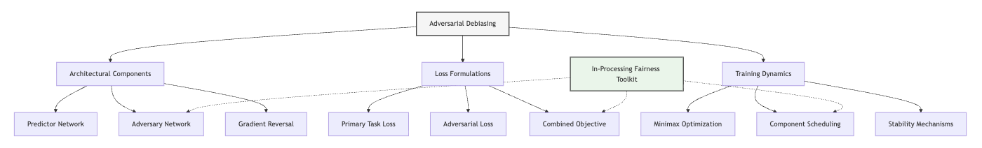
Adversarial Network Architecture for Fairness

Adversarial debiasing employs a network architecture with competing components designed to achieve fairness through a form of "representational protection." This concept is essential for fairness because it enables models to learn representations that are simultaneously predictive of the target variable and independent of protected attributes, effectively preventing problematic patterns from being encoded within the model.

The core architectural paradigm, inspired by Generative Adversarial Networks (GANs), involves two primary components:

A predictor that attempts to accurately predict the target variable Y from input features X
An adversary that attempts to predict the protected attribute A from either the predictor's output or internal representations

These components are trained with opposing objectives: the predictor aims to maximize prediction accuracy while minimizing the adversary's ability to infer protected attributes. This creates a minimax game where the equilibrium solution represents a model that achieves high accuracy while ensuring protected attributes cannot be recovered from its predictions or representations.

Zhang et al. (2018) formalized this approach in their seminal paper "Mitigating Unwanted Biases with Adversarial Learning," demonstrating how adversarial techniques could implement various fairness definitions. Their research showed that by carefully designing the adversarial objective, models could achieve demographic parity, equalized odds, or equal opportunity while maintaining competitive predictive performance.

The architectural design has significant implications for both fairness and implementation. As Beutel et al. (2017) demonstrated, different architectural choices—such as whether the adversary operates on the model's internal representations or final outputs—lead to different fairness properties and training dynamics. These choices must be aligned with specific fairness definitions and application requirements.

For the In-Processing Fairness Toolkit you'll develop in Unit 5, understanding these architectural patterns is crucial for determining when and how to implement adversarial approaches across different model types and fairness definitions.

Fairness Through Adversarial Unlearning

Adversarial debiasing achieves fairness through a process that can be conceptualized as "adversarial unlearning"—actively removing information about protected attributes from model representations while preserving predictive power. This mechanism is fundamentally different from constraint-based approaches and offers unique capabilities for balancing fairness and performance.

This concept connects to representational fairness, which focuses on what information is encoded within a model's internal states rather than just its outputs. By preventing the model from encoding protected attributes in its representations, adversarial methods address a deeper form of fairness than approaches that merely constrain output distributions.

As demonstrated by Edwards and Storkey (2016) in their work on fair representations, adversarial training can create "censored representations" that are simultaneously informative for the prediction task and uninformative about protected attributes. Their research showed that this approach could effectively remove protected attribute information from intermediate representations while maintaining high performance on the primary task.

The key insight is that adversarial unlearning operates by creating a form of information bottleneck that filters out protected attribute information. This filtering happens dynamically during training, as the predictor learns to encode features in ways that the adversary cannot exploit to infer protected attributes.

One significant advantage of this approach is its flexibility across different model architectures. While constraint-based methods often require specific mathematical formulations tied to model types, adversarial unlearning can be applied to virtually any differentiable model, from simple linear classifiers to complex neural networks.

For your In-Processing Fairness Toolkit, understanding this unlearning mechanism will help you determine when adversarial approaches offer advantages over other fairness techniques, particularly for complex models where protected attribute information might be encoded in subtle, non-linear ways.

Optimization Dynamics and Training Stability

Implementing adversarial debiasing requires careful attention to optimization dynamics and training stability. While conceptually elegant, adversarial training introduces significant challenges due to the competing objectives and potential for unstable dynamics during the learning process.

This concept is critical for practical implementation because naive adversarial training often suffers from instability issues, including oscillating behavior, mode collapse, or failure to converge to meaningful solutions. Understanding and addressing these challenges is essential for developing effective fairness interventions.

Research by Louppe et al. (2017) on adversarial learning demonstrates that the minimax game between predictor and adversary creates a fundamentally different optimization landscape than standard supervised learning. Their work reveals that the saddle-point nature of the objective function requires specialized training procedures to ensure stable convergence to desirable solutions.

Key optimization considerations include:

Balancing component strength: If the adversary becomes too powerful too quickly, the predictor may struggle to learn useful representations; conversely, if the adversary is too weak, fairness objectives may not be enforced.
Gradient reversal: Implemented through a special layer that multiplies gradients by a negative constant during backpropagation, effectively allowing the predictor to minimize the primary loss while maximizing the adversary's loss.
Progressive training schedules: Gradually increasing the weight of the adversarial component during training, allowing the predictor to first learn useful representations before enforcing fairness constraints.
Regularized adversarial objectives: Adding regularization terms to the adversarial objective to promote stability and prevent pathological solutions.

Research by Madras et al. (2018) demonstrated that implementing these techniques correctly is essential for achieving both fairness and performance goals. Their empirical studies showed that without proper optimization strategies, adversarial methods could lead to models that are either unfair or perform poorly on the primary task.

For the In-Processing Fairness Toolkit, understanding these optimization dynamics will enable you to provide practical guidance on implementing stable and effective adversarial training across different fairness definitions and model architectures.

Domain Modeling Perspective

From a domain modeling perspective, adversarial debiasing maps to specific components of ML systems:

Model Architecture: Adversarial debiasing requires specific architectural designs with competing components and information flow patterns.
Loss Function Design: The approach employs complex loss functions that balance primary task performance against protected attribute predictability.
Representation Learning: Adversarial mechanisms specifically target how information is encoded in model representations.
Optimization Process: The competing objectives create unique training dynamics requiring specialized optimization approaches.
Fairness Evaluation: Measuring both task performance and protected attribute leakage becomes essential for assessing effectiveness.

This domain mapping helps you understand how adversarial techniques influence different aspects of model development rather than viewing them as isolated modifications. The In-Processing Fairness Toolkit will leverage this mapping to guide appropriate technique selection and implementation across different modeling contexts.

Conceptual Clarification

To clarify these abstract adversarial concepts, consider the following analogies:

Adversarial debiasing functions like a sophisticated information filter system in a classified document environment. The primary classifier (predictor) tries to extract meaningful information for authorized purposes, while a security auditor (adversary) continuously monitors whether protected information is leaking through. When the auditor detects protected information, the classifier's methodology is adjusted to filter it out. Over time, this adversarial relationship creates a classifier that can extract useful information while provably protecting sensitive details—similar to how adversarial debiasing produces models that make accurate predictions while protecting sensitive attributes.
The minimax game in adversarial debiasing resembles a basketball training scenario where a shooter practices against an increasingly adaptive defender. The shooter (predictor) aims to score baskets (accurate predictions) while the defender (adversary) tries to block shots based on reading the shooter's patterns. When the defender successfully anticipates the shooter's moves by recognizing patterns related to protected attributes, the shooter must develop new techniques that remain effective but don't reveal these patterns. The equilibrium is reached when the shooter can score consistently while the defender cannot predict shots based on protected characteristics.
Optimization dynamics in adversarial training are similar to teaching two students with carefully balanced incentives. One student (the predictor) receives points for correct answers but loses points if they use certain prohibited shortcuts. Another student (the adversary) earns points specifically by catching the first student using these shortcuts. If the second student becomes too good too quickly, the first student may give up entirely; if the second student is ineffective, the first student will rely on shortcuts. The teacher must carefully adjust the reward structure and training pace to ensure both students improve appropriately—just as developers must carefully manage adversarial training dynamics to achieve both fairness and performance.

Intersectionality Consideration

Adversarial debiasing must explicitly address how multiple protected attributes interact to create unique fairness challenges at demographic intersections. Traditional implementations often train separate adversaries for each protected attribute, potentially missing complex discriminatory patterns that operate at intersections.

As Crenshaw (1989) established in her foundational work, discrimination often manifests differently at intersections of multiple identities, creating unique challenges that single-attribute analyses miss. For AI systems, this means adversarial approaches must be designed to prevent discrimination not just against individual protected groups but also against specific intersectional subgroups.

Recent work by Subramanian et al. (2021) demonstrates how adversarial architectures can be extended to address intersectionality by:

Designing adversaries that predict combinations of protected attributes rather than individual attributes
Implementing multi-task adversaries that simultaneously predict multiple protected attributes
Employing hierarchical adversarial structures that address both individual attributes and their intersections
Developing adversarial objectives that explicitly penalize discrimination against intersectional subgroups

Their research shows that these approaches can significantly improve fairness at demographic intersections compared to standard adversarial implementations that address protected attributes independently.

For the In-Processing Fairness Toolkit, addressing intersectionality requires explicit architectural and optimization considerations that extend beyond single-attribute approaches. Your framework should guide practitioners in implementing adversarial techniques that protect all demographic subgroups, including those at intersections that might otherwise receive inadequate protection from standard implementations.

3. Practical Considerations

Implementation Framework

To effectively implement adversarial debiasing in practice, follow this structured methodology:

Architectural Design:
Select an appropriate base architecture for the predictor component based on your primary task requirements.
Design the adversary architecture with complexity proportional to the difficulty of protected attribute prediction.
Implement a gradient reversal layer or equivalent mechanism between predictor and adversary.
Establish appropriate information flow connections based on your fairness definition:
- For demographic parity: Connect the adversary to the predictor's output
- For equalized odds: Connect the adversary to both the predictor's output and the true labels
- For representation fairness: Connect the adversary to the predictor's internal representations
Loss Function Formulation:
Define the primary task loss (e.g., cross-entropy for classification, mean squared error for regression).
Formulate the adversarial loss (typically cross-entropy for protected attribute prediction).
Construct the combined objective with appropriate weighting:
```
L_combined = L_primary - λ * L_adversarial
```
Implement a schedule for the adversarial weight λ that increases gradually during training.
Training Procedure:
Initialize both predictor and adversary components with appropriate weights.
Implement a progressive training schedule:
- Begin with a low weight for the adversarial component (small λ)
- Gradually increase λ as training progresses
- Potentially employ alternating optimization phases if stability issues arise
Monitor both primary task performance and protected attribute leakage throughout training.
Implement early stopping based on a combined metric that balances performance and fairness.

These methodologies integrate with standard ML workflows by extending conventional training procedures with additional components and objectives. While they add complexity to model development, they provide powerful fairness guarantees that may be difficult to achieve through other approaches.

Implementation Challenges

When applying adversarial debiasing, practitioners commonly face several challenges:

Training Instability: Adversarial training often suffers from instability due to competing objectives. Address this by:
Implementing gradient penalty terms that promote smoother optimization landscapes
Using progressive training schedules with careful learning rate management
Monitoring loss trajectories for signs of instability (e.g., oscillation, mode collapse)
Employing techniques like spectral normalization to stabilize adversary training
Architecture Balancing: The relative capacity of predictor and adversary significantly affects outcomes. Address this by:
Ensuring the adversary is powerful enough to learn protected attributes if they are present
Preventing the adversary from becoming too powerful too quickly, which can destabilize training
Experimenting with different architectural complexities to find an appropriate balance
Implementing regularization that prevents either component from dominating

Successfully implementing adversarial debiasing requires computational resources for training and monitoring multiple network components, expertise in adversarial training techniques, and patience for the experimental tuning often needed to achieve stable and effective results.

Evaluation Approach

To assess whether your adversarial debiasing implementation is effective, implement these evaluation strategies:

Protected Attribute Leakage Testing:
Train separate "probe" classifiers that attempt to predict protected attributes from model outputs or representations
Calculate mutual information between protected attributes and model representations
Compare leakage metrics before and after adversarial training
Test leakage across intersectional demographic categories, not just main groups
Fairness-Performance Trade-off Analysis:
Plot Pareto frontiers showing the trade-off between primary task performance and fairness metrics
Identify knee points on these frontiers that represent optimal trade-offs
Compare adversarial results with those from other fairness approaches (constraints, regularization)
Calculate the "price of fairness" in terms of performance reduction per fairness improvement

These evaluation approaches should be integrated with your organization's broader fairness assessment framework, providing specialized metrics for adversarial techniques while enabling comparison with alternative fairness interventions.

4. Case Study: Resume Screening System

Scenario Context

A large corporation is developing an automated resume screening system to help their HR department process the high volume of job applications they receive. The system analyzes resume text and work history to predict candidate suitability for different roles, producing a "qualification score" that helps prioritize applications for human review.

Initial testing revealed concerning disparities: the system consistently assigned lower qualification scores to female candidates compared to males with similar qualifications. Further analysis showed this bias stemmed partly from the training data (historical hiring decisions that favored men) and partly from the system learning to associate gender-correlated language patterns with qualification.

The data science team wants to implement fairness interventions while maintaining the system's ability to identify truly qualified candidates. They've already tried pre-processing approaches (modifying training data to balance gender representation), but these interventions either insufficiently addressed the bias or significantly reduced model performance.

The team decides to explore adversarial debiasing as an in-processing approach that might better balance fairness and performance. They face several challenges: the complex neural network architecture makes constraint-based methods difficult to implement; the text-based inputs create subtle patterns that correlate with gender; and they need to ensure fairness across intersectional categories (gender, race, age) while maintaining strong predictive performance.

Problem Analysis

Applying adversarial debiasing concepts to this scenario reveals several key considerations:

Architectural Design: The resume screening system uses a neural network with text embeddings as input features. An adversarial approach would require adding an adversary network that attempts to predict applicant gender from either the qualification score (for demographic parity) or both the score and the ground truth qualification label (for equalized odds).
Protected Information Pathways: Gender information enters the system in multiple ways:
Explicit indicators (e.g., women's colleges, gender-specific organizations)
Implicit patterns in language use (e.g., different adjective choices documented in research)
Employment gaps or part-time work that correlate with gender due to social factors
Educational backgrounds that correlate with gender due to historical patterns
Adversarial Objective: The team needs to decide which fairness definition best suits their goals. Demographic parity would ensure equal qualification rate distributions across genders, while equalized odds would ensure equal true positive and false positive rates, potentially better preserving the system's ability to identify truly qualified candidates.
Intersectional Considerations: Testing revealed that bias was particularly pronounced for certain intersectional groups, such as women over 40 and women from certain ethnic backgrounds. A standard adversarial approach addressing only gender might fail to protect these specific intersectional groups.

The key challenge is designing an adversarial system that effectively removes gender information from qualification predictions while maintaining the model's ability to identify truly qualified candidates based on legitimate qualification signals.

Solution Implementation

To address these challenges through adversarial debiasing, the team implemented a structured approach:

Architectural Implementation:
They designed a base neural network with text embedding inputs, followed by several hidden layers that produce the qualification score.
They added an adversary network connected to both the qualification score output and intermediate representations from the base network.
They implemented a gradient reversal layer between the main network and the adversary to enable the minimax training process.
They designed the adversary to predict not just gender, but also intersectional categories (combinations of gender, age range, and ethnicity).
Loss Function Formulation:
Primary loss: Binary cross-entropy based on historical hiring decisions (qualified/not qualified)
Adversarial loss: Multi-task loss predicting protected attributes (gender, age range, ethnicity, and their intersections)
Combined objective: L_combined = L_primary - λ * L_adversarial
Progressive weighting: Starting with λ = 0.1 and gradually increasing to 1.0 during training
Training Implementation:
They initialized both networks with pre-trained weights from a standard resume screening model.
They implemented a progressive training schedule that gradually increased the adversarial component weight.
They monitored both qualification prediction accuracy and protected attribute leakage throughout training.
They used early stopping based on a combined metric that balanced qualification prediction performance against fairness metrics.
Evaluation and Tuning:
They evaluated demographic parity by measuring differences in average qualification scores across gender groups.
They assessed equalized odds by measuring differences in true positive and false positive rates.
They tested for intersectional fairness by examining score distributions across different demographic subgroups.
They iteratively adjusted the adversarial weight and architecture based on these evaluations.

Throughout implementation, they maintained explicit focus on intersectional effects, ensuring that the adversarial component prevented discrimination not just against women overall but against specific intersectional groups that were particularly vulnerable to bias.

Outcomes and Lessons

The adversarial implementation produced significant improvements compared to both the original biased model and alternative fairness interventions:

The qualification score gap between male and female candidates decreased by 87%, substantially better than the 62% reduction achieved through pre-processing.
The system maintained 92% of its original performance in identifying truly qualified candidates, compared to only 84% when using constraint-based approaches.
Intersectional fairness improvements were more consistent than with other methods, with qualification score gaps decreasing by at least 75% across all demographic subgroups.

Key challenges included:

Initial training instability that required careful tuning of learning rates and component scheduling
Finding the right balance between the complexity of the adversary and main network
Determining the optimal weight for the adversarial component (λ) to balance fairness and performance

The most generalizable lessons included:

Architecture matters significantly: The specific design of the adversary and its connections to the main network dramatically affected both fairness and stability.
Progressive training is crucial: Starting with a small adversarial weight and gradually increasing it produced much better results than using a fixed weight throughout training.
Explicit intersectional design is necessary: Adversaries designed to protect specific intersectional groups performed substantially better than those targeting only primary demographic categories.
Representation protection is powerful: Connecting the adversary to internal representations as well as outputs provided stronger fairness guarantees than output-only connections.

These insights directly inform the development of the In-Processing Fairness Toolkit in Unit 5, particularly in creating guidance for implementing effective adversarial debiasing across different model types and fairness definitions.

5. Frequently Asked Questions

FAQ 1: Adversarial Vs. Constraint-Based Approaches

Q: When should I use adversarial debiasing instead of the constraint-based approaches covered in Unit 1, and what are the key trade-offs between these methods?
A: Adversarial debiasing typically offers advantages over constraint-based approaches when working with complex models, non-convex objectives, or when flexibility in fairness-performance trade-offs is important. The key differences include: First, architectural compatibility - adversarial methods work naturally with neural networks and other complex architectures where explicit constraints are difficult to formulate or enforce, making them ideal for deep learning models. Second, optimization flexibility - adversarial approaches typically provide smoother trade-offs between fairness and performance compared to hard constraints, allowing more granular control through the adversarial weight parameter. Third, representational fairness - adversarial methods can protect internal representations, not just outputs, potentially addressing deeper forms of bias that constraints might miss. However, adversarial approaches generally require more computational resources, introduce greater training complexity, and offer weaker theoretical guarantees than constraint methods. Choose adversarial debiasing when working with neural networks, dealing with complex inputs like text or images, or when you need to fine-tune the fairness-performance balance. Prefer constraint-based approaches when working with simpler models (linear, convex), when strong theoretical guarantees are required, or when computational resources are limited.

FAQ 2: Implementation Stability Challenges

Q: My adversarial debiasing implementation is unstable during training, with oscillating losses and inconsistent results. What practical techniques can improve stability without sacrificing fairness or performance?
A: Training instability is a common challenge with adversarial methods, but several practical techniques can significantly improve stability: First, implement progressive scheduling - start with a very small adversarial weight (λ ≈ 0.01) and gradually increase it following a schedule (linear, exponential, or sigmoid), which allows the primary task to establish good representations before enforcing fairness. Second, use learning rate asymmetry - typically set the adversary's learning rate to be 2-5× lower than the predictor's rate to prevent oscillations; if the adversary becomes too powerful too quickly, training will destabilize. Third, apply gradient clipping and normalization to prevent extreme gradient values that can derail training. Fourth, consider pretraining the primary model without the adversary, then freezing earlier layers while fine-tuning with adversarial components. Fifth, implement spectral normalization on the adversary to limit its capacity and promote Lipschitz continuity, which significantly improves stability. Sixth, monitor both losses during training and implement early stopping with a patience mechanism that triggers when oscillations become severe. Finally, consider alternating update schedules where you update the predictor and adversary in separate phases rather than simultaneously. These techniques often need to be combined and tuned for your specific model, but together they can transform an unstable implementation into a reliable training process.

6. Project Component Development

Component Description

In Unit 5, you will develop the adversarial debiasing section of the In-Processing Fairness Toolkit. This component will provide structured guidance for selecting, implementing, and optimizing adversarial approaches across different model architectures and fairness definitions.

The deliverable will include architectural patterns for different fairness goals, implementation templates with stability mechanisms, and decision criteria for determining when adversarial approaches are most appropriate compared to other in-processing techniques.

Development Steps

Create Architectural Pattern Templates: Develop standardized architectural patterns for implementing adversarial debiasing across different model types and fairness definitions. Include specific patterns for demographic parity, equalized odds, and representation fairness, with variations for different base architectures (feed-forward networks, CNNs, RNNs, transformers).
Design Implementation Guidance: Create practical implementation templates with code patterns for gradient reversal, loss function formulation, and progressive training schedules. Include specific guidance on hyperparameter selection, component balance, and stability mechanisms.
Develop Selection Criteria: Build decision frameworks for determining when adversarial approaches are more appropriate than constraints, regularization, or multi-objective methods. Create comparison matrices highlighting the strengths, limitations, and appropriate use cases for each approach.

Integration Approach

This adversarial component will interface with other parts of the In-Processing Fairness Toolkit by:

Building on the constraint-based approaches from Unit 1, positioning adversarial methods as alternatives particularly suited for complex models.
Establishing connections to the regularization approaches from Unit 3, highlighting how adversarial and regularization techniques can be combined.
Providing inputs to the multi-objective optimization approaches in Unit 4, showing how adversarial objectives can be incorporated into explicit trade-off formulations.

To enable successful integration, clearly document the interfaces between adversarial and other approaches, including when they complement each other versus when they offer alternative implementation paths. Develop consistent terminology and evaluation metrics across components to facilitate comparison and integration.

7. Summary and Next Steps

Key Takeaways

This Unit has explored the powerful paradigm of adversarial debiasing for incorporating fairness directly into model training. Key insights include:

Architectural design is fundamental to adversarial debiasing, with competing networks structured to prevent discrimination while maintaining predictive performance. The specific connections between predictor and adversary components determine which fairness properties are enforced.
Adversarial unlearning provides a distinctive approach to fairness by actively removing protected attribute information from model representations rather than simply constraining outputs. This enables deeper fairness protections, particularly for complex models.
Training dynamics require careful management to achieve both stability and effectiveness. Techniques like progressive scheduling, gradient reversal, and component balancing are essential for successful implementation.
Intersectional fairness demands explicit consideration in adversarial approaches, with specialized architectures and objectives needed to protect overlapping demographic groups.

These concepts directly address our guiding questions by demonstrating how adversarial techniques can prevent models from encoding discriminatory patterns while maintaining performance, and by establishing the architectural and optimization principles that enable effective implementation.

Application Guidance

To apply these concepts in your practical work:

Start by analyzing whether your model architecture and fairness requirements align well with adversarial approaches. Complex models with representational bias are typically good candidates.
Design your adversarial architecture carefully, ensuring the adversary connects to the appropriate predictor outputs or representations based on your specific fairness definition.
Implement progressive training schedules that gradually increase the adversarial weight, allowing the primary task to establish good representations before enforcing fairness constraints.
Monitor both primary task performance and protected attribute leakage throughout training, using these metrics to tune the adversarial weight and architecture.

If you're new to adversarial techniques, begin with simpler architectural designs and gradually incorporate more advanced features like multi-task adversaries or representation protection as you gain experience. Start with small adversarial weights (λ ≈ 0.1) and conservative learning rates to ensure training stability while you learn the dynamics of these systems.

Looking Ahead

In the next Unit, we will explore regularization approaches to fairness, which offer a more flexible alternative to both constraints and adversarial methods. You will learn how carefully designed penalty terms can guide models toward fairer solutions without the complexity of adversarial training or the rigidity of constraints.

The adversarial techniques you've learned in this Unit complement these regularization approaches in important ways. While adversarial methods excel at preventing protected attribute information from being encoded in representations, regularization can more easily target specific fairness metrics directly. By understanding both approaches, you'll be equipped to select the most appropriate technique for your specific modeling context and fairness requirements.

References

Beutel, A., Chen, J., Zhao, Z., & Chi, E. H. (2017). Data decisions and theoretical implications when adversarially learning fair representations. Proceedings of the Conference on Fairness, Accountability, and Transparency in Machine Learning (FAT/ML).

Crenshaw, K. (1989). Demarginalizing the intersection of race and sex: A black feminist critique of antidiscrimination doctrine, feminist theory and antiracist politics. University of Chicago Legal Forum, 1989(1), 139-167.

Edwards, H., & Storkey, A. (2016). Censoring representations with an adversary. International Conference on Learning Representations (ICLR).

Louppe, G., Kagan, M., & Cranmer, K. (2017). Learning to pivot with adversarial networks. Advances in Neural Information Processing Systems, 30.

Madras, D., Creager, E., Pitassi, T., & Zemel, R. (2018). Learning adversarially fair and transferable representations. International Conference on Machine Learning, 3384-3393.

Subramanian, S., Chakraborty, S., & Slotta, J. (2021). Fairness through adversarially learned debiasing. Proceedings of the AAAI/ACM Conference on AI, Ethics, and Society, 386-396.

Zhang, B. H., Lemoine, B., & Mitchell, M. (2018). Mitigating unwanted biases with adversarial learning. Proceedings of the 2018 AAAI/ACM Conference on AI, Ethics, and Society, 335-340.

Unit 3

Unit 3: Regularization for Fairness

1. Conceptual Foundation and Relevance

Guiding Questions

Question 1: How can fairness objectives be incorporated into model training as regularization terms rather than strict constraints, and what advantages does this flexibility provide?
Question 2: What trade-offs emerge when balancing fairness regularization against model performance, and how can these be navigated effectively in practical applications?

Conceptual Context

Regularization for fairness represents a pivotal approach in the fairness intervention taxonomy, offering a middle ground between the rigid structure of constraint-based methods and the potential insufficiency of pre-processing techniques. While constraint-based approaches (Unit 1) enforce strict fairness criteria that models must satisfy, regularization instead guides models toward fairness by penalizing unfair behaviors during training—creating a smoother optimization landscape that allows for more nuanced trade-offs.

This flexibility is particularly valuable because real-world fairness problems rarely have perfect solutions. As Corbett-Davies and Goel (2018) note, strict fairness constraints can sometimes lead to "fairness gerrymandering," where a model satisfies formal fairness criteria while still producing harmful outcomes. Regularization provides a more adaptable framework that can be calibrated to specific contexts, allowing practitioners to navigate the inherent tensions between competing fairness definitions and performance objectives.

The regularization approach builds directly on the optimization foundations established in Unit 1 and complements the adversarial techniques explored in Unit 2. Where constraints create hard boundaries that optimization cannot cross, regularization establishes soft penalties that can be balanced against the primary objective. This creates a continuous spectrum of solutions rather than a binary distinction between "fair" and "unfair" models, enabling more graceful degradation of performance when pursuing fairness.

Understanding regularization for fairness will directly inform the In-Processing Fairness Toolkit you'll develop in Unit 5, providing essential techniques for cases where constraint flexibility is needed but architectural modifications for adversarial approaches are impractical.

2. Key Concepts

Fairness as Regularization Penalty

Regularization transforms fairness criteria from hard constraints into penalty terms that the model tries to minimize alongside its primary objective. This conceptual shift is fundamental because it reframes fairness as a continuous goal rather than a binary property, allowing for more nuanced optimization that accounts for the inevitable trade-offs in real-world applications.

In standard machine learning, regularization typically penalizes model complexity to prevent overfitting. Fairness regularization extends this concept by adding penalty terms that measure disparities across protected groups, guiding the model away from discriminatory behaviors while still allowing it to find the best possible balance with performance objectives.

This concept directly connects to the optimization framework established in Unit 1, where we examined fairness as constraints. It also interacts with the adversarial approaches from Unit 2 by providing an alternative, often more stable mechanism for incorporating fairness into the training process. While adversarial methods create an implicit penalty through competition, regularization makes this penalty explicit in the objective function.

Kamishima et al. (2012) pioneered this approach with their prejudice remover regularizer, which penalizes mutual information between predictions and protected attributes. Their work demonstrated how such regularization can effectively reduce discrimination while maintaining reasonable predictive performance. For classification tasks, their regularizer takes the form:

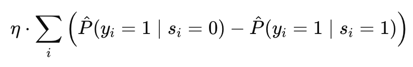
where η controls the strength of the fairness penalty relative to the primary objective, and the summation measures prediction disparities across protected groups.

Building on this foundation, Bechavod and Ligett (2017) developed more generalized fairness regularizers that can implement various fairness definitions, including demographic parity and equalized odds. Their approach allows practitioners to select regularization terms that align with their specific fairness goals while maintaining a unified optimization framework.

For the In-Processing Fairness Toolkit you'll develop in Unit 5, understanding fairness regularization is essential because it provides a flexible technique that can be implemented across diverse model architectures and learning algorithms. This flexibility makes regularization particularly valuable when rigid constraints are impractical or when balancing multiple competing objectives.

Regularization Parameter Tuning

The regularization parameter (λ or η in most formulations) controls the balance between the primary objective (typically prediction accuracy) and fairness goals. This parameter serves as a crucial control point that allows practitioners to navigate the fairness-performance frontier according to application requirements. Tuning this parameter effectively is fundamental to successful fairness regularization.

This concept builds on the basic formulation of fairness regularization by focusing on how to calibrate the strength of fairness penalties. It interacts with multi-objective optimization (which we'll explore in Unit 4) by providing a simple yet powerful mechanism for balancing competing goals without requiring explicit multi-objective frameworks.

Research by Hardt et al. (2016) demonstrates how parameter tuning creates a continuous spectrum of solutions with different fairness-performance trade-offs. As the regularization parameter increases, models typically sacrifice some predictive performance to achieve greater fairness. This creates a Pareto frontier of solutions rather than a single "optimal" model, allowing practitioners to select operating points based on domain-specific requirements and constraints.

The parameter tuning process typically involves:

Training models with different regularization strengths
Evaluating both performance and fairness metrics for each model
Selecting the parameter value that achieves the best trade-off for the specific application

This approach provides significant advantages over constraint-based methods, which typically offer less control over trade-offs. As Zafar et al. (2017) note, "Regularization allows practitioners to explore the entire fairness-accuracy spectrum rather than restricting them to solutions that satisfy rigid thresholds."

For the In-Processing Fairness Toolkit, parameter tuning strategies will be essential components that enable adaptive fairness interventions. By understanding how to effectively calibrate regularization strength, you'll be able to guide model development toward solutions that appropriately balance fairness against other critical objectives based on specific application contexts.

Group-Specific Regularization

Standard fairness regularizers typically apply uniform penalties across all protected groups. However, research increasingly shows that effective fairness interventions often require group-specific approaches that account for the different ways bias manifests across demographics. Group-specific regularization extends basic fairness penalties by applying different regularization strengths or forms to different protected groups.

This concept builds on the foundational idea of fairness regularization by adding greater nuance and specificity. It interacts with intersectionality (which we'll explore further in Unit 4) by providing mechanisms for addressing the unique fairness challenges that arise at demographic intersections.

Lahoti et al. (2020) demonstrated the value of group-specific regularization in their work on individual fairness. They introduced an approach that adaptively applies stronger regularization to traditionally disadvantaged groups, focusing fairness interventions where they're most needed rather than applying uniform penalties that might unnecessarily degrade performance for well-represented groups.

Similarly, Kearns et al. (2018) showed how subgroup-specific regularization can address "fairness gerrymandering," where models appear fair across broad demographics but exhibit significant disparities at intersections. Their approach applies targeted regularization to intersectional subgroups, preventing models from achieving superficial fairness by compensating for discrimination against specific intersections with favoritism toward others.

Group-specific regularization typically takes forms such as:

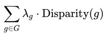
where G represents the set of protected groups, λg is a group-specific regularization strength, and Disparity(g) measures unfairness for group g.

For the In-Processing Fairness Toolkit, group-specific regularization provides essential techniques for addressing complex fairness challenges involving multiple protected attributes or intersectional considerations. By incorporating these approaches, you'll develop a framework capable of addressing nuanced fairness requirements rather than just broad demographic parity.

Fairness-Accuracy Trade-off Analysis

Fairness regularization inevitably creates trade-offs with predictive performance, as models must balance fairness penalties against their primary optimization objectives. Understanding and analyzing these trade-offs is crucial for effective implementation of regularization approaches, enabling informed decisions about appropriate operating points.

This concept builds on parameter tuning by focusing on the analytical framework for evaluating trade-offs rather than just the mechanism for creating them. It directly connects to multi-objective optimization (Unit 4) by providing the empirical foundation for more formal approaches to trade-off navigation.

Research by Kleinberg et al. (2016) established theoretical limits to these trade-offs, demonstrating that certain fairness criteria cannot be simultaneously satisfied when base rates differ across groups. Building on this theoretical work, Menon and Williamson (2018) provided practical frameworks for analyzing the Pareto frontier of fairness-accuracy trade-offs, enabling quantitative evaluation of different operating points.

A typical trade-off analysis involves:

Training models with varying regularization strengths
Plotting performance metrics against fairness metrics
Identifying "knees" in the curve where marginal fairness improvements require disproportionate performance sacrifices
Selecting operating points that balance competing priorities based on application requirements

This analysis provides crucial insights that inform regularization parameter selection. As Agarwal et al. (2018) note, "Understanding the shape of the fairness-accuracy Pareto frontier is often more valuable than finding a single 'optimal' solution, as it enables context-specific decisions about acceptable trade-offs."

For the In-Processing Fairness Toolkit, trade-off analysis methodologies will be essential components that enable informed decision-making about regularization implementation. By incorporating these approaches, you'll develop a framework that not only implements fairness regularization but also provides the analytical tools to evaluate its effects and select appropriate configurations.

Domain Modeling Perspective

From a domain modeling perspective, fairness regularization connects to specific components of ML systems:

Objective Function: Fairness regularizers add penalty terms directly to the optimization objective, creating a modified loss function that the model minimizes during training.
Loss Calculation: The training process computes fairness penalties alongside the primary loss, creating a combined signal that guides optimization.
Gradient Updates: During backpropagation, parameter updates are influenced by both performance and fairness gradients, steering the model toward solutions that balance these objectives.
Hyperparameter Configuration: Regularization strengths are tuned alongside other hyperparameters, creating a fairness-aware model selection process.
Evaluation Framework: Trade-off analysis requires expanding traditional evaluation to include both performance and fairness metrics, creating a multi-dimensional assessment framework.

This domain mapping helps you understand how regularization integrates with different aspects of the model development process rather than viewing it as an isolated technique. The In-Processing Fairness Toolkit will leverage this mapping to guide appropriate technique implementation across different modeling workflows.

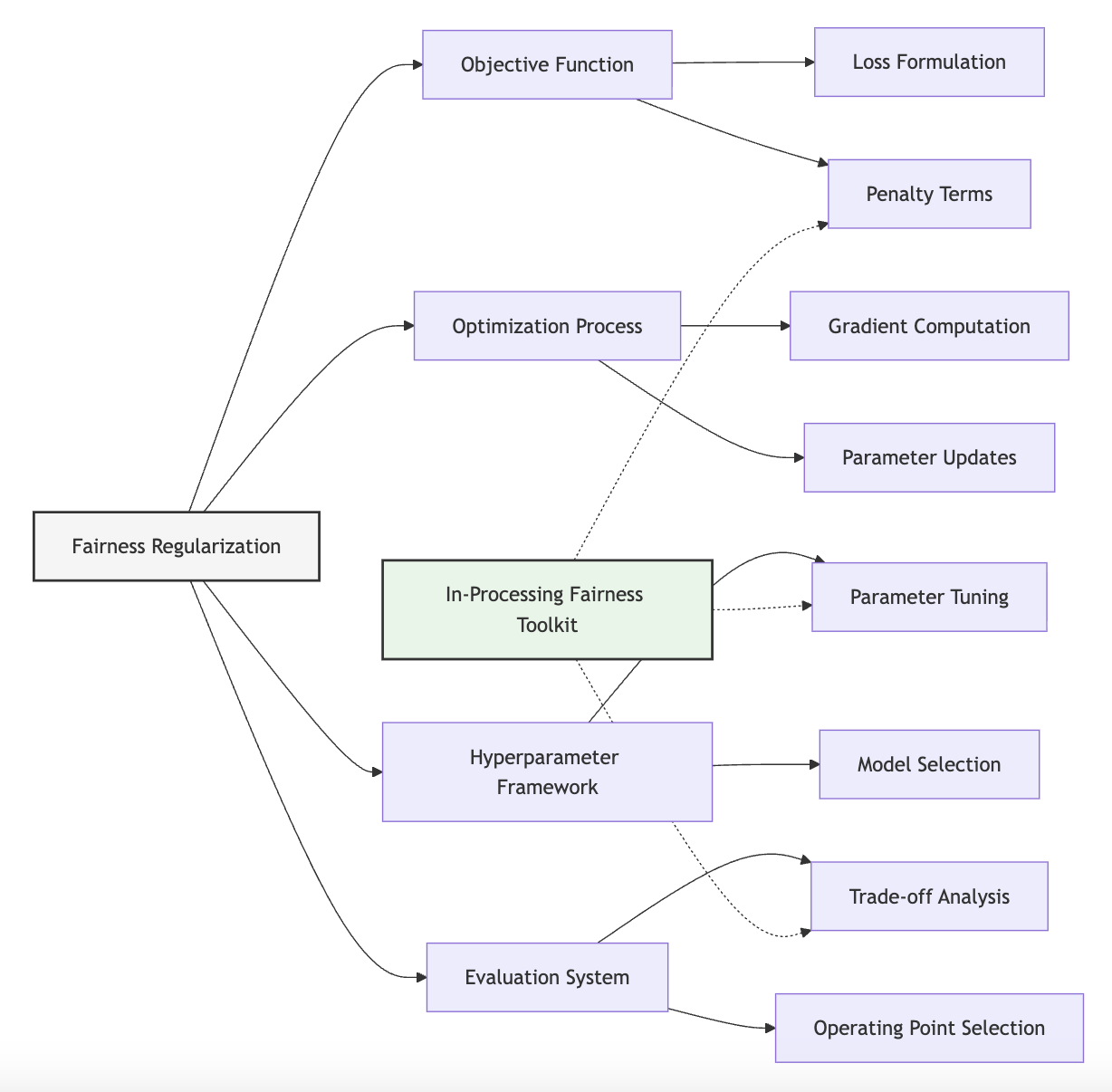
Conceptual Clarification

To clarify these abstract regularization concepts, consider the following analogies:

Fairness regularization is similar to progressive taxation in economic policy, where behaviors are discouraged through financial penalties rather than outright prohibitions. Just as tax policy might impose higher rates on activities a society wants to limit without banning them entirely, regularization imposes computational costs on unfair model behaviors without strictly prohibiting them. This approach creates incentives that guide the model toward fairer solutions while maintaining flexibility when perfect fairness would be excessively costly or impossible.
Regularization parameter tuning resembles adjusting the thermostat in a building's climate control system. Setting the thermostat too low prioritizes energy efficiency but might leave occupants uncomfortable; setting it too high prioritizes comfort but wastes energy. Similarly, setting regularization parameters too low prioritizes predictive performance but permits unfairness; setting them too high prioritizes fairness but may unnecessarily sacrifice performance. The optimal setting depends on the specific context—a hospital might prioritize patient comfort over efficiency, just as a high-risk application might prioritize fairness over marginal performance gains.
Group-specific regularization functions like a progressive tax system with targeted deductions for disadvantaged groups. Rather than applying identical rates to everyone regardless of circumstances, such systems adjust burdens based on specific situations and needs. Similarly, group-specific regularization applies different fairness pressures based on the unique challenges facing different demographic groups, creating more nuanced interventions that focus resources where they're most needed.

Intersectionality Consideration

Traditional fairness regularizers often address protected attributes independently, potentially missing unique challenges at demographic intersections where multiple forms of discrimination combine. Effective regularization must account for these intersectional effects by penalizing unfairness across all relevant demographic combinations, not just main groups.

As Crenshaw (1989) established in her foundational work, discrimination often operates differently at the intersections of multiple marginalized identities, creating unique challenges that single-attribute approaches miss. For ML fairness, this means regularization techniques must address potential "fairness gerrymandering," where models appear equitable across broad demographics while discriminating against specific intersectional subgroups.

Kearns et al. (2018) formalized this challenge in their work on subgroup fairness, demonstrating that standard fairness approaches (including basic regularization) can allow significant discrimination against intersectional subgroups while maintaining fairness for broader categories. Their research showed that addressing this issue requires regularization terms that specifically account for performance across all relevant demographic combinations.

For example, a model might show similar aggregate performance for men and women, and similar aggregate performance across racial groups, while still performing poorly specifically for women of certain racial backgrounds. Addressing this requires regularization terms that specifically penalize disparities at these intersections rather than just across main demographic categories.

Implementing intersectional regularization typically involves:

Identifying relevant demographic intersections
Formulating regularization terms that specifically penalize disparities at these intersections
Weighting these penalties appropriately based on subgroup sizes and vulnerability
Evaluating fairness across both main groups and intersectional subgroups

For the In-Processing Fairness Toolkit, addressing intersectionality requires extending basic regularization approaches to capture intersectional effects, even when subgroup sample sizes are limited. This might involve techniques like hierarchical regularization that shares statistical strength across related subgroups while still capturing unique intersectional patterns.

3. Practical Considerations

Implementation Framework

To effectively implement fairness regularization in practice, follow this structured methodology:

Regularizer Design:
Formulate penalty terms that capture relevant fairness definitions (demographic parity, equalized odds, etc.).
For classification tasks, implement disparity measures based on prediction differences across groups.
For regression tasks, implement fairness penalties based on error distribution differences or correlation measures.
Ensure regularizers are differentiable to enable gradient-based optimization.
Integration with Learning Algorithms:
For linear/logistic regression: Add fairness terms directly to the objective function alongside traditional L1/L2 regularization.
For tree-based methods: Modify splitting criteria to incorporate fairness penalties during tree construction.
For neural networks: Implement custom loss functions that include fairness regularization terms.
Ensure compatibility with existing optimization approaches (SGD, Adam, etc.).
Parameter Tuning Strategy:
Implement grid search or Bayesian optimization over regularization strengths.
Use nested cross-validation to estimate generalization performance for different parameter values.
Create fairness-performance curves that visualize trade-offs across the parameter spectrum.
Select operating points based on application-specific requirements and constraints.
Evaluation Framework:
Assess both predictive performance and fairness metrics at each operating point.
Compare regularization results against constraint-based approaches to evaluate flexibility benefits.
Analyze potential disparate impacts across intersectional subgroups.
Document trade-offs explicitly to support informed decision-making.

These methodologies integrate with standard ML workflows by extending existing regularization frameworks rather than introducing entirely new paradigms. While adding analytical complexity, they work within familiar optimization processes and can often be implemented with minimal modifications to existing code.

Implementation Challenges

When implementing fairness regularization, practitioners commonly face these challenges:

Non-Convexity in Optimization: Many fairness regularizers introduce non-convexity into the objective function, potentially creating optimization difficulties. Address this by:
Starting with convex approximations of fairness metrics when possible.
Implementing robust optimization techniques like momentum-based methods.
Using warm-starting from less-regularized solutions to find better optima.
Experimenting with multiple random initializations to avoid poor local minima.
Balancing Multiple Fairness Criteria: Real applications often involve multiple fairness definitions that may conflict with each other. Address this by:
Creating composite regularizers that combine multiple fairness criteria with appropriate weights.
Implementing Pareto optimization to identify solutions that aren't dominated on any objective.
Using hierarchical approaches that prioritize critical fairness constraints while treating others as softer regularization.
Documenting trade-offs between competing fairness definitions to support informed decisions.

Successfully implementing fairness regularization requires resources including expertise in optimization techniques, computational capacity for parameter tuning, and domain knowledge for interpreting trade-offs. While more accessible than adversarial approaches, effective regularization still requires thoughtful implementation and evaluation.

Evaluation Approach

To assess whether your fairness regularization is effective, implement these evaluation strategies:

Fairness-Performance Trade-off Analysis:
Plot performance metrics (accuracy, AUC, etc.) against fairness metrics for models with different regularization strengths.
Identify Pareto-optimal solutions where no other model dominates on both dimensions.
Calculate the marginal cost of fairness—how much performance is sacrificed for each unit of fairness improvement.
Compare trade-off curves across different regularization formulations to identify superior approaches.
Generalization Assessment:
Evaluate fairness not just on the training data but on held-out validation sets.
Analyze stability of fairness improvements across different data splits.
Implement stratified cross-validation to ensure reliable evaluation across demographic groups.
Test robustness to distribution shifts that might affect fairness properties.

These evaluation approaches should be integrated with your organization's broader model validation framework, providing multi-dimensional assessment that includes fairness alongside traditional performance metrics.

4. Case Study: Loan Approval Algorithm

Scenario Context

A financial institution wants to develop a machine learning model to predict loan default risk, which will inform approval decisions and interest rates. Historical lending data is available, including applicant demographics, financial history, and loan outcomes. However, preliminary analysis reveals disparities in approval rates across racial and gender groups that cannot be fully explained by default risk differences.

The institution aims to develop a model that accurately predicts default risk while ensuring fair treatment across demographic groups. They've determined that demographic parity (similar approval rates across groups) and equal opportunity (similar approval rates for qualified applicants across groups) are both relevant fairness criteria, but they're concerned about the potential impact on the model's ability to accurately assess risk.

This scenario involves multiple stakeholders with different priorities: risk managers focused on predicting defaults accurately, compliance officers concerned about regulatory requirements, business leaders interested in maintaining profitability, and customers from diverse backgrounds seeking fair assessment.

Problem Analysis

Applying fairness regularization concepts to this scenario reveals several considerations:

Fairness-Performance Trade-offs: Initial experiments with constraint-based approaches showed that strictly enforcing demographic parity would increase expected defaults by approximately 12%, creating significant business impact. However, completely ignoring fairness concerns could create legal and reputational risks, as well as perpetuating historical inequities.
Multiple Fairness Criteria: The institution wants to balance multiple fairness definitions—demographic parity addresses historical underrepresentation in lending, while equal opportunity focuses on fair treatment of qualified applicants. These definitions sometimes pull the model in different directions, creating tensions that strict constraints struggle to resolve.
Group-Specific Considerations: Detailed analysis revealed different patterns of disadvantage across demographic groups. While some groups faced clear underrepresentation in approvals, others showed more subtle disparities in interest rate assignments or documentation requirements. This complexity suggested the need for group-specific fairness approaches rather than uniform constraints.

From an intersectional perspective, the challenges became even more nuanced. The data showed that women from certain racial backgrounds faced unique disadvantages that weren't fully captured by examining either gender or race independently. This suggested the need for regularization approaches that specifically addressed these intersectional effects.

Regularization offered a promising middle ground between ignoring fairness concerns and imposing strict constraints that might significantly impact performance. By incorporating fairness penalties into the objective function, the institution could guide the model toward more equitable predictions while maintaining the flexibility to balance multiple considerations.

Solution Implementation

The team implemented a comprehensive fairness regularization approach:

Regularizer Design: They formulated a composite regularizer that combined demographic parity and equal opportunity components:

def fairness_regularizer(y_pred, protected_attrs, y_true):
    # Demographic parity component
    dp_penalty = disparate_impact_penalty(y_pred, protected_attrs)

    # Equal opportunity component (for qualified applicants)
    qualified = (y_true == 0)  # non-defaulting applicants
    eo_penalty = equal_opp_penalty(y_pred, protected_attrs, qualified)

    # Combine with weights reflecting priorities
    return lambda_dp * dp_penalty + lambda_eo * eo_penalty

Integration with Learning Algorithm: Since they were using gradient boosting for the risk model, they implemented the regularizer by modifying the split-finding criterion:

def regularized_split_criterion(gradient, hessian, protected_attrs):
    # Standard split criterion
    standard_gain = compute_split_gain(gradient, hessian)

    # Fairness penalty for this split
    fairness_penalty = compute_split_fairness_impact(gradient, protected_attrs)

    # Combined criterion
    return standard_gain - lambda_fairness * fairness_penalty

Parameter Tuning: They conducted extensive experiments with different regularization strengths, creating a Pareto frontier of solutions:
λ = 0: Achieved 85% accuracy with significant demographic disparities (18% approval gap)
λ = 0.1: Reduced the approval gap to 12% with minimal accuracy impact (84%)
λ = 0.5: Further reduced the gap to 7% with moderate accuracy impact (82%)
λ = 1.0: Achieved near-parity (3% gap) but with more substantial accuracy decline (79%)
Group-Specific Approach: They implemented different regularization strengths for different demographic intersections, focusing stronger regularization on groups with historical disadvantages:

def group_specific_regularizer(y_pred, race, gender, income_level):
    # Base regularization for all groups
    penalty = base_fairness_penalty(y_pred, race, gender)

    # Additional penalties for specific intersectional groups
    for group in high_priority_groups:
        indices = get_group_indices(race, gender, income_level, group)
        penalty += additional_group_penalty(y_pred, indices, group['lambda'])

    return penalty

Trade-off Analysis: They created detailed visualizations showing the relationship between different metrics:
Performance metrics: Accuracy, expected profit, risk coverage
Fairness metrics: Demographic parity difference, equal opportunity difference
Business impact metrics: Expected defaults, approval rates

This analysis enabled stakeholders to understand the concrete implications of different operating points and make informed decisions about an appropriate balance.

Outcomes and Lessons

The regularization approach yielded several key benefits:

Balanced Solution: The institution selected a regularization strength (λ = 0.3) that reduced approval disparities by 65% while sacrificing only 2% in accuracy. This operating point represented a "knee" in the Pareto curve where additional fairness gains would require disproportionate performance sacrifices.
Flexible Implementation: Unlike constraint-based approaches, regularization allowed the model to make appropriate exceptions when legitimate risk factors strongly indicated default likelihood, while still broadly improving fairness metrics.
Transparent Trade-offs: The fairness-performance curves provided clear documentation of the implications of different fairness priorities, facilitating informed decision-making and regulatory discussions.
Intersectional Improvements: The group-specific approach successfully addressed unique challenges facing intersectional subgroups, reducing maximum disparities at demographic intersections by 72%.

Key challenges included computational complexity of parameter tuning, particularly for group-specific regularization, and communicating nuanced trade-offs to non-technical stakeholders.

The most generalizable lessons included:

The importance of extensive trade-off analysis rather than selecting a single "optimal" fairness parameter.
The value of group-specific approaches that focus stronger regularization on historically disadvantaged groups.
The need to balance multiple fairness criteria rather than optimizing for a single definition.
The benefit of regularization's flexibility compared to strict constraints, particularly for applications with complex risk considerations.

These insights directly inform the In-Processing Fairness Toolkit in Unit 5, demonstrating how regularization provides a flexible and effective approach to incorporating fairness into the learning process while navigating inevitable trade-offs.

5. Frequently Asked Questions

FAQ 1: Regularization Vs. Constraints

Q: When should I use fairness regularization instead of the constraint-based approaches covered in Unit 1?
A: Fairness regularization offers several advantages over constraints that make it more suitable in specific contexts: First, regularization provides greater flexibility when perfect fairness is unattainable or would severely impact performance. While constraints create hard boundaries that might render optimization infeasible or force excessive performance sacrifices, regularization creates smoother penalties that permit graceful trade-offs. Second, regularization often leads to more stable optimization, particularly for complex models like deep neural networks where constrained optimization can cause training instability or convergence issues. Third, regularization enables easier balancing of multiple, potentially conflicting fairness criteria by assigning them different weights in a composite penalty term, whereas handling multiple constraints often requires more complex formulations. Finally, regularization integrates more naturally with existing training workflows, requiring minimal modifications to standard optimization procedures. Choose regularization when you need to balance fairness against other objectives, when working with complex models where constraints cause optimization difficulties, when addressing multiple fairness criteria simultaneously, or when you need to explore the entire fairness-performance frontier rather than a single operating point.

FAQ 2: Parameter Tuning Strategies

Q: What practical approaches help identify appropriate regularization strengths without exhaustive grid search?
A: While grid search across regularization values provides comprehensive coverage, several more efficient approaches can help identify appropriate regularization strengths: Begin with Bayesian optimization, which intelligently samples the parameter space based on previous results, typically finding good configurations with fewer trials than grid search. Implement log-scale exploration by testing regularization strengths across orders of magnitude (0.001, 0.01, 0.1, 1, 10) to quickly identify promising regions before fine-tuning. Consider warm-starting, where you train with gradually increasing regularization strengths, using each model to initialize the next—this often converges faster and finds better optima than training each configuration from scratch. For complex scenarios involving multiple fairness criteria, try random sampling with budget allocation, testing random parameter combinations but allocating more budget to promising regions. Finally, incorporate domain knowledge by starting with values based on subject matter expertise about acceptable trade-offs in your specific application. Regardless of approach, always analyze the shape of the fairness-performance curve rather than just selecting the "best" parameter—understanding the trade-off landscape often proves more valuable than identifying a single operating point, as it enables contextual decision-making based on specific application requirements.

6. Project Component Development

Component Description

In Unit 5, you will develop the regularization section of the In-Processing Fairness Toolkit. This component will provide structured guidance for implementing fairness regularization across different model types, including regularizer formulations, integration patterns, parameter tuning approaches, and trade-off analysis methodologies.

The deliverable will include regularization templates for common model architectures, implementation patterns for different learning algorithms, tuning strategies for navigating the fairness-performance frontier, and evaluation frameworks for assessing regularization effectiveness.

Development Steps

Create Regularizer Formulation Templates: Develop mathematical formulations and implementation patterns for different fairness regularizers, covering demographic parity, equalized odds, and other relevant definitions. Include implementation examples for classification and regression contexts.
Design Algorithm Integration Patterns: Build integration approaches for incorporating fairness regularizers into different learning algorithms, including gradient-based methods, tree-based approaches, and probabilistic models. Provide code templates and architecture-specific guidelines.
Develop Parameter Tuning Methodologies: Create systematic approaches for calibrating regularization strengths, including grid search strategies, Bayesian optimization frameworks, and multi-objective tuning. Include tools for visualizing and analyzing the fairness-performance frontier.

Integration Approach

This regularization component will interface with other parts of the In-Processing Fairness Toolkit by:

Building on the fairness objectives from Unit 1, showing how to transform constraints into regularization terms.
Complementing the adversarial approaches from Unit 2, providing alternatives when architectural modifications are impractical.
Establishing foundations for the multi-objective optimization in Unit 4, showing how regularization offers a simpler approach to balancing competing goals.

To enable successful integration, document clear decision criteria for choosing between constraints, regularization, and adversarial approaches based on model characteristics and application requirements. Develop consistent interfaces that allow regularization techniques to be combined with other approaches when appropriate.

7. Summary and Next Steps

Key Takeaways

This Unit has explored how fairness can be effectively incorporated into model training through regularization approaches. Key insights include:

Fairness as Penalty: Regularization transforms fairness criteria from hard constraints into penalty terms that the model tries to minimize alongside its primary objective, creating a continuous spectrum of solutions rather than a binary fair/unfair distinction.
Flexible Trade-offs: The regularization parameter (λ) provides a crucial control point for navigating the fairness-performance frontier, allowing practitioners to make context-appropriate trade-offs rather than enforcing rigid thresholds.
Group-Specific Approaches: Different demographic groups often face unique challenges that require tailored interventions, making group-specific regularization particularly valuable for addressing intersectional fairness concerns.
Trade-off Analysis: Understanding the shape of the fairness-performance Pareto frontier is often more valuable than finding a single "optimal" solution, as it enables informed decisions based on application requirements.

These concepts directly address our guiding questions by demonstrating how fairness objectives can be incorporated as regularization terms and how the resulting trade-offs can be effectively navigated through parameter tuning and comprehensive analysis.

Application Guidance

To apply these concepts in your practical work:

Start by formulating appropriate regularizers based on your specific fairness definitions, ensuring they're differentiable for gradient-based optimization.
Implement these regularizers within your existing model training workflow, using custom loss functions or modified optimization objectives.
Conduct parameter tuning experiments to map the fairness-performance frontier, testing multiple regularization strengths.
Create visualization tools that help stakeholders understand the trade-offs between competing objectives.
Document your regularization approach, including formulation choices, parameter selection rationale, and trade-off analysis.

If you're new to fairness regularization, begin with simpler formulations like demographic parity penalties for classification tasks, which are straightforward to implement and interpret. As you gain experience, you can progress to more sophisticated approaches like intersectional regularization or composite penalties that balance multiple fairness criteria.

Looking Ahead

In the next Unit, we will build on this foundation of regularization to explore multi-objective optimization for fairness. While regularization provides an implicit approach to balancing competing objectives through penalty weights, multi-objective optimization offers more formal frameworks for navigating these trade-offs.

The regularization concepts you've learned here will provide essential background for understanding multi-objective approaches. Where regularization combines objectives into a single weighted sum, multi-objective optimization explicitly models the Pareto frontier of solutions, enabling more principled exploration of the trade-off space. This progression from regularization to multi-objective frameworks completes our exploration of in-processing techniques before we develop the comprehensive Integration Framework in Unit 5.

References

Agarwal, A., Beygelzimer, A., Dudík, M., Langford, J., & Wallach, H. (2018). A reductions approach to fair classification. In Proceedings of the 35th International Conference on Machine Learning (pp. 60-69).

Bechavod, Y., & Ligett, K. (2017). Penalizing unfairness in binary classification. arXiv preprint arXiv:1707.00044.

Corbett-Davies, S., & Goel, S. (2018). The measure and mismeasure of fairness: A critical review of fair machine learning. arXiv preprint arXiv:1808.00023.

Crenshaw, K. (1989). Demarginalizing the intersection of race and sex: A black feminist critique of antidiscrimination doctrine, feminist theory and antiracist politics. University of Chicago Legal Forum, 140, 139-167.

Hardt, M., Price, E., & Srebro, N. (2016). Equality of opportunity in supervised learning. In Advances in Neural Information Processing Systems (pp. 3315-3323).

Kamishima, T., Akaho, S., Asoh, H., & Sakuma, J. (2012). Fairness-aware classifier with prejudice remover regularizer. In Joint European Conference on Machine Learning and Knowledge Discovery in Databases (pp. 35-50). Springer.

Kearns, M., Neel, S., Roth, A., & Wu, Z. S. (2018). Preventing fairness gerrymandering: Auditing and learning for subgroup fairness. In International Conference on Machine Learning (pp. 2564-2572).

Kleinberg, J., Mullainathan, S., & Raghavan, M. (2016). Inherent trade-offs in the fair determination of risk scores. arXiv preprint arXiv:1609.05807.

Lahoti, P., Gummadi, K. P., & Weikum, G. (2020). Operationalizing individual fairness with pairwise fair representations. Proceedings of the VLDB Endowment, 13(4), 506-518.

Menon, A. K., & Williamson, R. C. (2018). The cost of fairness in binary classification. In Conference on Fairness, Accountability and Transparency (pp. 107-118).

Zafar, M. B., Valera, I., Gomez Rodriguez, M., & Gummadi, K. P. (2017). Fairness constraints: Mechanisms for fair classification. In Artificial Intelligence and Statistics (pp. 962-970).

Zhang, B. H., Lemoine, B., & Mitchell, M. (2018). Mitigating unwanted biases with adversarial learning. In Proceedings of the 2018 AAAI/ACM Conference on AI, Ethics, and Society (pp. 335-340).

Unit 4

Unit 4: Multi-Objective Optimization

1. Conceptual Foundation and Relevance

Guiding Questions

Question 1: How can we systematically navigate the inherent tensions between fairness criteria and traditional performance metrics in machine learning model development?
Question 2: What methodologies enable principled trade-off decisions rather than ad hoc compromises when multiple, potentially conflicting objectives must be balanced?

Conceptual Context

When implementing fairness in machine learning systems, you inevitably encounter a fundamental challenge: fairness objectives often conflict with traditional performance metrics and sometimes even with other fairness criteria. While the constraint-based and regularization approaches from previous Units offer ways to incorporate fairness into model training, they typically treat fairness as a secondary consideration to performance or rely on manual tuning of hyperparameters to balance competing objectives.

Multi-objective optimization provides a more principled framework for navigating these inherent tensions. Rather than treating fairness as a constraint or penalty term in a primarily performance-focused objective, multi-objective approaches explicitly model the trade-offs between different objectives, allowing for systematic exploration of solution spaces and informed decision-making about acceptable compromises.

This perspective is particularly vital in high-stakes applications where both fairness and performance are critical considerations. As Agarwal et al. (2019) note, "The trade-offs inherent in fair machine learning are not merely technical artifacts but reflect fundamental societal values that must be explicitly considered rather than implicitly embedded in algorithm design."

This Unit builds directly on the fairness objectives and constraints from Unit 1, the adversarial frameworks from Unit 2, and the regularization approaches from Unit 3, showing how these techniques can be incorporated into comprehensive multi-objective frameworks. The insights developed here will directly inform the In-Processing Fairness Toolkit you'll develop in Unit 5, providing methodologies for explicitly modeling trade-offs and selecting appropriate compromise solutions across diverse modeling contexts.

2. Key Concepts

The Fairness-Performance Trade-off

Implementing fairness in machine learning systems typically involves trade-offs with traditional performance metrics such as accuracy, precision, or recall. This relationship is not merely an implementation artifact but reflects fundamental theoretical limitations. Understanding these trade-offs is essential for designing systems that appropriately balance different objectives.

Corbett-Davies et al. (2017) rigorously demonstrated that enforcing fairness constraints often comes at a measurable cost to traditional performance metrics. Their analysis of risk assessment tools showed that imposing fairness constraints like demographic parity or equal opportunity necessarily reduced overall accuracy when the base rates of positive outcomes differed across groups—a common scenario in real-world applications.

This trade-off exists because fairness constraints effectively restrict the model's capacity to leverage all available predictive information, particularly when that information correlates with protected attributes. For instance, enforcing demographic parity in a loan approval system might require ignoring legitimately predictive features that happen to correlate with protected attributes, potentially reducing the model's ability to accurately predict default risk.

The fairness-performance trade-off interacts with other concepts by establishing why multi-objective frameworks are necessary in the first place. Unlike optimization problems with a single clear objective, fairness-aware machine learning involves fundamentally competing goals that cannot be simultaneously optimized to their individual maxima. This inherent tension necessitates explicit modeling of trade-offs rather than implicit handling through hyperparameter tuning.

For the In-Processing Fairness Toolkit, understanding these trade-offs is essential for designing systems that make principled compromises based on application requirements rather than arbitrary decisions that may unknowingly sacrifice critical objectives.

Pareto Optimality in Fairness Contexts

When optimizing for multiple competing objectives, we need a framework for understanding which solutions represent reasonable compromises. Pareto optimality provides such a framework by defining solutions where no objective can be improved without degrading another. This concept is fundamental to multi-objective optimization for fairness, as it helps identify the set of reasonably balanced solutions.

A solution is Pareto optimal if no other solution exists that would improve at least one objective without degrading any other. The set of all Pareto optimal solutions forms the Pareto frontier, which represents the fundamental trade-offs inherent in the problem.

Martinez et al. (2020) demonstrated the application of Pareto optimality to fairness-performance trade-offs, showing how different fairness definitions create distinct Pareto frontiers with varying impacts on traditional performance metrics. Their work illustrated how explicitly modeling these frontiers enables more informed decision-making compared to ad hoc parameter tuning.

For example, in a credit scoring application, the Pareto frontier might consist of models ranging from those maximizing accuracy with no fairness considerations to those achieving perfect demographic parity at the cost of reduced predictive performance, with various compromise solutions in between. Each point on this frontier represents a model where accuracy cannot be improved without increasing unfairness, and fairness cannot be improved without decreasing accuracy.

This concept interacts with previously covered approaches by providing a framework for understanding the space of possible solutions when using constraints, adversarial methods, or regularization. Instead of treating these techniques as distinct approaches, Pareto optimality allows us to view them as different ways of navigating the same fundamental trade-off space.

For the In-Processing Fairness Toolkit, Pareto optimality will provide a theoretical foundation for comparing different fairness implementations and selecting appropriate operating points based on application requirements.

Scalarization Methods

To navigate the Pareto frontier effectively, we need practical methods for finding specific Pareto optimal solutions that represent appropriate compromises. Scalarization methods convert multi-objective problems into single-objective problems by combining multiple objectives into a scalar (single-value) objective function, providing concrete ways to implement multi-objective fairness optimization.

Linear scalarization combines objectives through weighted sums, where the weights reflect the relative importance of different objectives. For example, a fairness-aware objective might take the form:

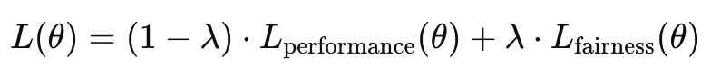
where λ ∈ [0, 1] controls the trade-off between performance and fairness.

As Zafar et al. (2019) demonstrate, different scalarization weights explore different points on the Pareto frontier. By systematically varying these weights, practitioners can generate a range of Pareto optimal solutions, enabling informed selection based on application requirements.

Alternative approaches include the ε-constraint method, which optimizes one objective while constraining others to be within acceptable bounds. This approach aligns well with scenarios where minimum performance or fairness thresholds must be maintained.

Scalarization connects to regularization approaches from Unit 3, as fairness regularization can be viewed as a specific form of scalarization with fixed weights. However, multi-objective frameworks extend this by explicitly exploring the full range of possible trade-offs rather than committing to a single weighting.

For the In-Processing Fairness Toolkit, scalarization methods provide practical implementation techniques for exploring and navigating the fairness-performance trade-off space, enabling the development of systems that balance competing objectives according to application-specific priorities.

Preference Articulation and Solution Selection

Once we've identified the Pareto frontier of possible fairness-performance trade-offs, we need methodologies for selecting specific solutions that align with application requirements and stakeholder values. Preference articulation provides frameworks for expressing priorities and selecting appropriate operating points from the range of Pareto optimal solutions.

Preference articulation can occur at different stages of the optimization process:

A priori articulation: Preferences are defined before optimization, typically through objective weights or constraints. This approach requires stakeholders to quantify their preferences before seeing potential solutions.
A posteriori articulation: A range of Pareto optimal solutions is generated first, then stakeholders select from this range after seeing the concrete trade-offs. This approach allows more informed decision-making but requires generating multiple solutions.
Interactive articulation: Preferences are refined iteratively as stakeholders explore the trade-off space, providing feedback that guides the search toward preferred regions of the Pareto frontier.

Research by Kleinberg et al. (2018) highlights how preference articulation in fairness contexts involves not just technical considerations but fundamental value judgments about what constitutes an appropriate balance between competing notions of fairness and performance. Their work demonstrates that these decisions cannot be made purely on technical grounds but require engagement with the normative aspects of fairness.

For example, in a hiring algorithm, stakeholders might initially specify equal importance for accuracy and demographic parity, then adjust these preferences after seeing that this balance results in unacceptable performance drops for certain positions. Through interactive articulation, they might discover that different fairness-performance balances are appropriate for different job categories.

This concept interacts with the fairness-performance trade-off by providing methodologies for navigating this trade-off space based on stakeholder values and application requirements. Rather than treating the trade-off as a purely technical challenge, preference articulation acknowledges the value-laden nature of these decisions.

For the In-Processing Fairness Toolkit, preference articulation will provide structured approaches for selecting specific operating points from the Pareto frontier based on application context and stakeholder priorities.

Domain Modeling Perspective

From a domain modeling perspective, multi-objective optimization for fairness maps to specific components of ML systems:

Objective Formulation: Multiple objectives (performance, various fairness criteria) are explicitly modeled rather than combined implicitly.
Solution Space Exploration: Techniques for generating diverse Pareto optimal solutions rather than single points.
Trade-off Visualization: Methods for representing multi-dimensional trade-off spaces to stakeholders.
Preference Modeling: Frameworks for capturing stakeholder priorities and value judgments.
Operating Point Selection: Decision processes for selecting specific solutions from the Pareto frontier.

This domain mapping helps you understand how multi-objective approaches transform the model development process rather than simply adding fairness as a secondary consideration. The In-Processing Fairness Toolkit will leverage this mapping to design comprehensive fairness implementation approaches that explicitly address trade-offs throughout the development lifecycle.

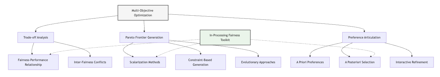
Conceptual Clarification

To clarify these abstract multi-objective concepts, consider the following analogies:

The fairness-performance trade-off is similar to fuel efficiency versus acceleration in automotive design. Just as a car cannot simultaneously maximize both fuel economy and rapid acceleration (due to fundamental physical constraints), a machine learning model cannot simultaneously maximize both traditional performance metrics and certain fairness criteria when base rates differ across groups. Automotive engineers explicitly model these trade-offs through Pareto curves that show the frontier of possible combinations, allowing car manufacturers to produce different models targeting different points on this spectrum—from fuel-efficient economy cars to high-performance sports cars. Similarly, ML practitioners can generate a range of models along the fairness-performance frontier, allowing application-specific selection based on requirements.
Pareto optimality in fairness resembles financial portfolio optimization where investors balance risk against return. Just as an investment portfolio is Pareto optimal if no other portfolio exists that would provide higher returns with the same risk or lower risk with the same returns, a machine learning model is Pareto optimal if no other model exists that would improve performance without reducing fairness or improve fairness without reducing performance. Investment advisors typically present clients with the efficient frontier of investment options, allowing them to select a portfolio matching their risk tolerance. Similarly, ML systems can present stakeholders with the fairness-performance frontier, enabling selection based on organizational priorities and fairness requirements.
Preference articulation functions like dietary planning that balances nutrition against taste preferences. Some people set strict nutritional requirements before considering taste (a priori articulation), others sample many foods and then select those that best balance nutrition and taste (a posteriori articulation), while still others iteratively refine their diet based on both nutritional feedback and taste experiences (interactive articulation). Similarly, organizations might set strict fairness requirements before considering performance, explore a range of models with different fairness-performance balances before selecting one, or interactively refine their preferences as they better understand the concrete trade-offs involved.

Intersectionality Consideration

Traditional multi-objective approaches often optimize fairness criteria for each protected attribute independently, potentially missing unique challenges at intersections of multiple identities. Effective multi-objective optimization must explicitly address intersectional fairness by including objectives that capture fairness across overlapping demographic categories.

As Buolamwini and Gebru (2018) demonstrated in their "Gender Shades" research, systems may achieve reasonable fairness metrics when evaluated on single attributes (e.g., gender or race separately) while showing significant disparities at their intersections (e.g., specific combinations of gender and race). This phenomenon creates additional complexity for multi-objective optimization, as the number of potential objectives increases combinatorially with the number of protected attributes considered.

Recent work by Foulds et al. (2020) proposes intersectional fairness objectives that explicitly model performance across all demographic subgroups rather than just main categories. Their approach ensures that multi-objective optimization addresses the unique challenges faced by individuals at demographic intersections, who might otherwise be overlooked in aggregated metrics.

For example, in a resume screening system, traditional multi-objective approaches might balance accuracy against gender fairness and racial fairness separately. An intersectional approach would explicitly include objectives for each combination of gender and race, ensuring that the system works fairly for Black women, Asian men, and other specific demographic intersections rather than just achieving fairness in aggregate gender and race metrics.

For the In-Processing Fairness Toolkit, addressing intersectionality requires:

Explicitly including intersectional fairness objectives in multi-objective formulations.
Developing visualization techniques that effectively communicate intersectional trade-offs to stakeholders.
Implementing preference articulation approaches that can handle the higher-dimensional objective spaces created by intersectional considerations.
Designing efficient optimization techniques that scale to the larger number of objectives without becoming computationally intractable.

By incorporating these intersectional considerations, the framework will enable more comprehensive fairness optimization that protects all demographic subgroups rather than just main categories.

3. Practical Considerations

Implementation Framework

To effectively apply multi-objective optimization for fairness in practice, follow this structured methodology:

Trade-off Analysis and Objective Definition:
Define the specific performance metrics (accuracy, F1-score, AUC, etc.) relevant to your application.
Specify the fairness criteria (demographic parity, equal opportunity, etc.) you need to satisfy.
Analyze potential conflicts between objectives through preliminary experiments or theoretical analysis.
Document the complete set of objectives with clear mathematical formulations and evaluation methodologies.
Pareto Frontier Exploration:
Implement scalarization methods with systematically varied weights to generate diverse solutions.

For linear scalarization, train models with different λ values in the combined objective:

def objective(model_params, lambda_val):    performance_loss = calculate_performance_loss(model_params)    fairness_loss = calculate_fairness_loss(model_params)    return (1 - lambda_val) * performance_loss + lambda_val * fairness_loss

Alternatively, implement the ε-constraint method by optimizing performance subject to varying fairness bounds.
Verify the Pareto optimality of generated solutions by confirming that no objective can be improved without degrading another.
Solution Evaluation and Visualization:
Calculate comprehensive metrics for each solution, including performance measures, fairness metrics, and relevant application-specific indicators.
Develop visualizations that effectively communicate trade-offs, such as:
- 2D plots for two-objective problems (e.g., accuracy vs. demographic parity)
- Parallel coordinate plots for higher-dimensional objective spaces
- Radar charts for comparing specific solutions across multiple metrics
Annotate visualizations with contextual information to aid interpretation, such as baseline performance or regulatory thresholds.
Preference Articulation and Selection:
For a priori articulation, encode stakeholder preferences as specific objective weights or constraints.
For a posteriori articulation, present the Pareto frontier to stakeholders and facilitate solution selection through interactive tools.
For interactive articulation, implement feedback mechanisms that refine the search based on stakeholder input.
Document selection rationales and the value judgments they reflect for accountability and future reference.

These methodologies integrate with standard ML workflows by extending model selection and hyperparameter tuning processes to explicitly consider multiple objectives. While they add analytical complexity, they provide a more principled approach to fairness implementation than ad hoc adjustments or implicit trade-offs.

Implementation Challenges

When implementing multi-objective optimization for fairness, practitioners commonly face these challenges:

Computational Complexity: Generating the Pareto frontier requires training multiple models, which can be resource-intensive. Address this by:
Using warm-starting techniques where solutions with similar objective weights share initialization parameters.
Implementing efficient approximation methods like evolutionary algorithms for large-scale problems.
Developing adaptive sampling strategies that focus computational resources on the most relevant regions of the Pareto frontier.
Leveraging transfer learning to adapt pre-trained models for different trade-off points rather than training from scratch.
High-Dimensional Objective Spaces: Problems with multiple fairness criteria and intersectional considerations create high-dimensional trade-off spaces that are difficult to explore and visualize. Address this by:
Using dimensionality reduction techniques to identify the most significant trade-offs.
Implementing progressive exploration that starts with primary objectives and incrementally incorporates additional dimensions.
Developing specialized visualization techniques for high-dimensional trade-offs.
Creating interactive tools that allow stakeholders to navigate complex trade-off spaces through guided exploration.

Successfully implementing multi-objective optimization for fairness requires resources including computational capacity for exploring diverse solutions, expertise in both machine learning and multi-objective optimization, and stakeholder engagement to guide the selection of appropriate operating points based on application-specific requirements.

Evaluation Approach

To assess whether your multi-objective fairness optimization is effective, implement these evaluation strategies:

Pareto Optimality Verification:
Conduct dominance analysis to confirm that generated solutions are not dominated by others (i.e., no solution exists that improves some objectives without degrading others).
Test for local improvements by perturbing solutions and verifying that no local adjustments can improve all objectives simultaneously.
Compare against baseline approaches to ensure that multi-objective solutions actually expand the range of available trade-offs.
Document verification results to demonstrate the quality of the generated Pareto frontier.
Hypervolume Assessment:
Calculate the hypervolume indicator, which measures the volume of the objective space dominated by your Pareto frontier.
Compare hypervolume against benchmark approaches to quantify the improvement in available trade-offs.
Track hypervolume growth during the optimization process to assess convergence.
Use hypervolume contribution to identify particularly valuable solutions in the Pareto set.
Stakeholder Satisfaction Evaluation:
Conduct structured assessments of whether the presented trade-offs meet stakeholder needs.
Evaluate the clarity and usefulness of trade-off visualizations for decision-making.
Measure the time and effort required for stakeholders to select appropriate operating points.
Document stakeholder feedback on the solution selection process to inform future improvements.

These evaluation approaches should be integrated with your organization's broader fairness assessment framework, providing a rigorous basis for determining whether multi-objective optimization effectively addresses the inherent tensions between fairness and performance in your specific application context.

4. Case Study: Lending Algorithm With Multiple Fairness Criteria

Scenario Context

A financial institution is developing a machine learning model to predict default risk for loan applications. The model analyzes credit history, income, employment stability, and other financial indicators to generate risk scores that inform lending decisions. Key stakeholders include the risk management team concerned with accurate default prediction, regulatory compliance officers monitoring fair lending practices, borrowers seeking equitable access to credit, and business leaders focused on portfolio performance.

The institution must navigate multiple fairness requirements: regulatory guidelines prohibit discrimination based on protected attributes like race and gender (requiring demographic parity), while business objectives demand accurate risk assessment (requiring predictive performance). Additionally, they want to ensure equal opportunity for creditworthy applicants across demographics. These objectives potentially conflict, particularly since creditworthiness indicators show different distributions across demographic groups due to historical inequities.

Problem Analysis

Applying multi-objective optimization concepts reveals several challenges in this lending scenario:

Inherent Trade-offs: Initial experiments show that enforcing strict demographic parity significantly reduces the model's ability to predict defaults accurately, as it restricts the use of legitimately predictive features that correlate with protected attributes. The risk team estimates a 15% reduction in predictive accuracy when strict demographic parity is enforced.
Competing Fairness Definitions: Equal opportunity (ensuring creditworthy applicants have equal approval chances regardless of protected attributes) and demographic parity (ensuring equal approval rates across demographic groups) sometimes conflict with each other. Analysis shows that achieving perfect demographic parity would require approving some higher-risk applications from certain demographics, potentially violating equal opportunity for truly low-risk applicants across all groups.
Intersectional Considerations: The fairness analysis becomes more complex when considering intersectional demographics. For instance, the model shows reasonable fairness metrics for gender and racial categories independently, but significant disparities emerge for specific combinations like younger women from certain racial backgrounds.
Stakeholder Tensions: Business leaders prioritize predictive accuracy to minimize default rates, while compliance officers emphasize demographic parity to meet regulatory requirements. Borrower advocates push for equal opportunity to ensure individuals are evaluated on their merits. These competing priorities cannot be simultaneously satisfied to their maximum extent.

Traditional approaches might address these challenges through ad hoc parameter tuning or selecting a single fairness criterion, potentially overlooking important trade-offs or failing to achieve an appropriate balance across objectives.

Solution Implementation

To address these challenges through multi-objective optimization, the team implemented a structured approach:

Objective Formulation:
They explicitly defined three objectives: predictive accuracy (measured by AUC), demographic parity (measured by the difference in approval rates across racial groups), and equal opportunity (measured by the difference in true positive rates across racial groups).
Each objective was formalized mathematically with clear evaluation metrics.
Pareto Frontier Generation:

The team implemented linear scalarization with systematically varied weights across the three objectives:

def multi_objective(model_params, w1, w2, w3):    accuracy_loss = 1 - calculate_auc(model_params)    demographic_parity_gap = calculate_approval_rate_difference(model_params)    equal_opportunity_gap = calculate_tpr_difference(model_params)    return w1 * accuracy_loss + w2 * demographic_parity_gap + w3 * equal_opportunity_gap

They trained models with different weight combinations, generating a diverse set of solutions across the trade-off space.
The team verified the Pareto optimality of these solutions by confirming that no objective could be improved without degrading another.
Trade-off Visualization:
They created interactive visualizations showing the three-dimensional trade-off space, highlighting the Pareto frontier.
For easier interpretation, they also generated two-dimensional projections focusing on specific trade-offs (e.g., accuracy vs. demographic parity).
They annotated these visualizations with regulatory thresholds and business performance requirements.
Solution Selection:
The team implemented a posteriori preference articulation, presenting the Pareto frontier to key stakeholders.
Through a structured decision process, stakeholders evaluated different operating points on the frontier.
They ultimately selected a solution that maintained 95% of the original predictive accuracy while reducing demographic parity differences to below regulatory thresholds and ensuring equal opportunity differences stayed below 5%.
Intersectional Considerations:
To address intersectional fairness, they extended their methodology to include objectives for key demographic intersections.
This required a higher-dimensional trade-off space but enabled more comprehensive fairness guarantees.
The selected solution was verified to maintain acceptable fairness metrics across both main demographic categories and their intersections.

Throughout implementation, the team maintained clear documentation of trade-offs, design decisions, and the rationales behind their choices, creating accountability and enabling future refinement.

Outcomes and Lessons

The multi-objective approach yielded several key benefits compared to traditional methods:

It provided explicit visibility into the trade-offs between predictive accuracy and different fairness criteria, enabling informed decision-making rather than implicit compromises.
The selected solution achieved a significantly better balance of objectives than either unconstrained optimization or single-fairness-criterion approaches.
The process created a structured framework for incorporating stakeholder preferences, transforming what was previously a contentious disagreement into a collaborative decision process based on concrete options.

Key challenges included the computational resources required to generate the Pareto frontier and the complexity of communicating multi-dimensional trade-offs to non-technical stakeholders. The team addressed these through efficient warm-starting techniques and carefully designed visualizations with contextual annotations.

The most generalizable lessons included:

The importance of explicitly modeling multiple objectives rather than combining them implicitly through constraints or penalties.
The value of generating and visualizing a diverse set of Pareto optimal solutions before committing to a specific trade-off.
The necessity of structured stakeholder engagement in selecting operating points from the Pareto frontier, recognizing that these choices reflect value judgments as much as technical considerations.

These insights directly inform the development of the In-Processing Fairness Toolkit in Unit 5, demonstrating how multi-objective optimization enables more principled fairness implementation compared to ad hoc approaches or single-criterion optimization.

5. Frequently Asked Questions

FAQ 1: Multi-Objective Optimization Vs. Regularization

Q: How does multi-objective optimization differ from fairness regularization, and when should I use one approach versus the other?
A: While regularization and multi-objective optimization both address fairness-performance trade-offs, they differ fundamentally in how they frame and navigate these trade-offs. Regularization incorporates fairness as a penalty term in a primarily performance-focused objective function, with a manually tuned hyperparameter controlling the fairness-performance balance. This approach implicitly navigates trade-offs through parameter tuning without explicitly modeling the full trade-off space. In contrast, multi-objective optimization explicitly models multiple objectives and systematically explores the Pareto frontier of possible trade-offs, enabling more informed selection based on a comprehensive understanding of available options. Use regularization when you need a simpler implementation with fewer computational requirements and already have a good intuition for the appropriate fairness-performance balance. Choose multi-objective optimization when you need to thoroughly understand the available trade-offs, when multiple stakeholders with different priorities must reach consensus, or when you must balance more than two objectives (e.g., multiple fairness criteria alongside performance). Multi-objective approaches require more computational resources but provide greater transparency and more principled navigation of complex trade-off spaces, particularly valuable in high-stakes applications where both fairness and performance are critical considerations.

FAQ 2: Handling Many Objectives

Q: How can I effectively implement multi-objective optimization when I have many fairness criteria across multiple protected attributes and their intersections?
A: Handling many objectives requires specialized approaches to avoid computational intractability and ensure meaningful results. First, conduct objective analysis to identify correlations between fairness metrics—some criteria may be highly correlated, allowing you to select representative metrics that implicitly address related concerns. Second, implement progressive preference articulation starting with primary objectives, then incorporating additional criteria as constraints once initial Pareto frontiers are established. This reduces the dimensionality of each optimization phase. Third, consider hierarchical approaches that group related objectives (e.g., organize metrics by protected attribute or fairness definition type) and optimize within groups before balancing across them. Fourth, leverage dimensionality reduction techniques like Principal Component Analysis to identify the most significant trade-off dimensions. Fifth, employ efficient many-objective optimization algorithms specifically designed for high-dimensional objective spaces, such as NSGA-III or reference-point based methods. Finally, develop specialized visualization techniques for high-dimensional trade-offs, such as heatmaps for intersectional metrics or interactive tools that allow stakeholders to explore specific slices of the objective space. When implementing these approaches, start with a reduced set of objectives to establish baseline trade-offs, then incrementally incorporate additional criteria as your understanding and computational capacity allow.

6. Project Component Development

Component Description

In Unit 5, you will develop the multi-objective optimization section of the In-Processing Fairness Toolkit. This component will provide a structured methodology for explicitly modeling trade-offs between fairness and performance objectives and selecting appropriate operating points based on application requirements and stakeholder priorities.

The deliverable will include techniques for generating Pareto optimal solutions, visualizing multi-dimensional trade-off spaces, and implementing preference articulation processes that enable informed selection from the range of available trade-offs.

Development Steps

Create a Multi-Objective Problem Formulation Guide: Develop a structured approach for translating fairness requirements and performance objectives into formal multi-objective optimization problems. Include templates for defining objectives, analyzing potential conflicts, and establishing evaluation metrics.
Design a Pareto Frontier Generation Framework: Build methodologies for efficiently generating diverse Pareto optimal solutions. Include implementation patterns for scalarization methods, constraint-based approaches, and evolutionary algorithms, with guidance on selecting appropriate techniques for different problem types.
Develop Trade-off Visualization and Selection Tools: Create approaches for effectively communicating multi-dimensional trade-offs to stakeholders and facilitating solution selection. Include visualization techniques for different objective configurations and preference articulation methodologies for different stakeholder contexts.

Integration Approach

This multi-objective component will interface with other parts of the In-Processing Fairness Toolkit by:

Building on the constraint-based approaches from Unit 1, the adversarial methods from Unit 2, and the regularization techniques from Unit 3, showing how these can be incorporated into multi-objective frameworks.
Providing a comprehensive approach for balancing multiple fairness criteria and performance objectives that complements the more focused techniques from previous Units.
Creating decision frameworks that help practitioners select appropriate techniques based on the specific trade-offs in their application context.

To enable successful integration, design the component with consistent terminology across framework elements, clear connections to other techniques, and implementation patterns that can be combined with the approaches from previous Units.

7. Summary and Next Steps

Key Takeaways

This Unit has explored how multi-objective optimization provides a principled framework for navigating the inherent tensions between fairness and performance in machine learning systems. Key insights include:

Trade-offs are inherent, not accidental: The tension between fairness and performance (and between different fairness criteria) reflects fundamental theoretical limits rather than implementation deficiencies. Multi-objective optimization makes these trade-offs explicit rather than hiding them in implementation details.
Pareto optimality provides a principled framework for understanding the space of reasonable compromise solutions, focusing attention on models where no objective can be improved without degrading another.
Scalarization methods offer practical implementation techniques for generating diverse Pareto optimal solutions, enabling exploration of the trade-off space through systematic variation of objective weights.
Preference articulation transforms technical trade-offs into value-based decisions, acknowledging that selecting operating points from the Pareto frontier involves fundamental value judgments about the relative importance of different objectives.

These concepts directly address our guiding questions by providing systematic methods for navigating fairness-performance tensions and enabling principled trade-off decisions rather than ad hoc compromises.

Application Guidance

To apply these concepts in your practical work:

Explicitly model multiple objectives rather than combining them implicitly through constraints or penalties, particularly when stakeholders have different priorities or when you need to balance several competing goals.
Generate and visualize diverse Pareto optimal solutions before committing to a specific trade-off, enabling informed selection based on a comprehensive understanding of available options.
Engage stakeholders in the solution selection process, recognizing that choosing operating points from the Pareto frontier reflects value judgments as much as technical considerations.
Document trade-offs and selection rationales to create accountability and enable future refinement as priorities evolve or new techniques become available.

For organizations new to multi-objective optimization, start with simpler two-objective problems (e.g., accuracy vs. demographic parity) before progressing to more complex multi-criteria scenarios. Use visualization tools to build intuition about trade-off spaces and develop stakeholder comfort with explicit trade-off navigation.

Looking Ahead

In the next Unit, we will synthesize all the techniques we've explored throughout this Part—constraint-based approaches, adversarial methods, regularization techniques, and multi-objective optimization—into a comprehensive In-Processing Fairness Toolkit. This framework will provide structured guidance for selecting and implementing appropriate in-processing techniques based on fairness definitions, model architectures, and practical constraints.

The multi-objective perspective you've developed in this Unit will be particularly valuable for the integration framework, as it provides a unifying paradigm for understanding how different in-processing techniques navigate the fundamental trade-offs inherent in fairness-aware machine learning. By viewing constraints, adversarial methods, and regularization as different ways of exploring the fairness-performance Pareto frontier, the framework will enable more coherent and principled technique selection.

References

Agarwal, A., Beygelzimer, A., Dudík, M., Langford, J., & Wallach, H. (2019). A reductions approach to fair classification. In Proceedings of the 35th International Conference on Machine Learning (pp. 60-69). http://proceedings.mlr.press/v80/agarwal18a.html

Buolamwini, J., & Gebru, T. (2018). Gender shades: Intersectional accuracy disparities in commercial gender classification. In Proceedings of the 1st Conference on Fairness, Accountability, and Transparency (pp. 77-91). https://proceedings.mlr.press/v81/buolamwini18a.html

Corbett-Davies, S., Pierson, E., Feller, A., Goel, S., & Huq, A. (2017). Algorithmic decision making and the cost of fairness. In Proceedings of the 23rd ACM SIGKDD International Conference on Knowledge Discovery and Data Mining (pp. 797-806). https://doi.org/10.1145/3097983.3098095

Foulds, J. R., Islam, R., Keya, K. N., & Pan, S. (2020). An intersectional definition of fairness. In 2020 IEEE 36th International Conference on Data Engineering (ICDE) (pp. 1918-1921). https://doi.org/10.1109/ICDE48307.2020.00203

Kleinberg, J., Ludwig, J., Mullainathan, S., & Rambachan, A. (2018). Algorithmic fairness. In AEA Papers and Proceedings (Vol. 108, pp. 22-27). https://doi.org/10.1257/pandp.20181018

Martinez, N., Bertran, M., & Sapiro, G. (2020). Minimax Pareto fairness: A multi objective perspective. In Proceedings of the 37th International Conference on Machine Learning (pp. 6755-6764). http://proceedings.mlr.press/v119/martinez20a.html

Valdivia, A., Sánchez-Monedero, J., & Casillas, J. (2021). How fair can we go in machine learning? Assessing the boundaries of fairness in decision trees. Knowledge-Based Systems, 215, 106775.

Zafar, M. B., Valera, I., Gomez-Rodriguez, M., & Gummadi, K. P. (2019). Fairness constraints: A flexible approach for fair classification. Journal of Machine Learning Research, 20(75), 1-42. http://jmlr.org/papers/v20/18-262.html

Unit 5

Unit 5: In-Processing Fairness Toolkit

1. Introduction

In Part 3, you learned about fairness constraints, adversarial debiasing, regularization approaches, and multi-objective optimization. Now build a toolkit that integrates fairness directly into model training. The In-Processing Fairness Toolkit serves as the third component of the Sprint 2 Project - Fairness Intervention Playbook. It moves beyond data pre-processing to embed fairness in the heart of your models.

2. Context

Imagine you're a staff engineer at a mid-sized bank, working with a team building a loan approval system. Pre-processing techniques have improved gender fairness, but gaps remain. The model still approves 70% of male applicants but only 62% of similarly qualified female applicants.

Their data science lead suspects the model needs fairness baked into its training process. She approaches you with questions: Which algorithms best constrain gender bias during training? Can adversarial methods help? How might these techniques affect model performance?

You've worked with the team through causal analysis and pre-processing. Now they need your guidance on integrating fairness directly into model training. You'll create an In-Processing Fairness Toolkit to guide their choices based on their model architecture, fairness goals, and technical constraints.

3. Objectives

By completing this project component, you will practice:

Analyzing model architectures for fairness compatibility.
Matching fairness definitions to specific algorithm constraints.
Implementing fairness techniques within model training loops.
Balancing fairness and predictive performance.
Translating mathematical constraints into actual code.
Verifying fairness improvements through rigorous testing.

4. Requirements

Your In-Processing Fairness Toolkit must include:

A Model Architecture Analysis Template identifying which techniques work with specific model types.
A Technique Selection Decision Tree guiding users from fairness goals to in-processing methods.
An Implementation Pattern Catalog providing reusable code templates.
An Integration Verification Framework validating fairness improvements.
User documentation explaining how to apply the toolkit.
A case study demonstrating the toolkit's application to a loan approval model.

5. Sample Solution

The following solution from a former colleague can serve as a starting point. Note that it lacks some key components your toolkit should include.

5.1 Model Architecture Analysis Template

This template analyzes model compatibility with fairness techniques:

Model Type Classification:

## Model Architecture Assessment
1. Model family:
   - Linear models (logistic regression, linear SVM)
   - Tree-based models (decision trees, random forests, gradient boosting)
   - Neural networks (feedforward, convolutional, recurrent)
   - Other (specify: ____________)

2. Model characteristics:
   - Training approach (batch, online, etc.)
   - Loss function
   - Regularization methods currently used
   - Hyperparameter tuning approach

3. Technical constraints:
   - Available computational resources
   - Maximum acceptable training time increase
   - Explainability requirements
   - Deployment environment limitations

Compatibility Matrix:

Fairness Technique	Linear Models	Tree-based Models	Neural Networks
Constraint Optimization	High	Low	Medium
Adversarial Debiasing	Low	Low	High
Fairness Regularization	High	Medium	High
Fair Representations	Medium	Low	High
Specialized Algorithms	Medium	High	Low

Implementation Considerations:

For each model type, document:

Technical limitations affecting fairness implementation
Modification approaches with least disruption
Performance impact expectations
Explainability implications

5.2 Technique Selection Decision Tree

This decision tree guides users to appropriate techniques:

Step 1: Model Architecture Assessment

What type of model are you using?
Linear model → Go to Step 2A
Tree-based model → Go to Step 2B
Neural network → Go to Step 2C
Other → Consider model-agnostic approaches

Step 2A: Linear Model Approaches

What is your primary fairness definition?
Demographic parity → Constraint optimization with optimization-based preprocessing
Equal opportunity → Constraint optimization with adjusted thresholds
Individual fairness → Similarity-based regularization

Step 2B: Tree-based Model Approaches

What is your primary fairness definition?
Demographic parity → Fair splitting criteria
Equal opportunity → Fair splitting with weighted samples
Individual fairness → Regularized tree induction

Step 2C: Neural Network Approaches

What is your primary fairness definition?
Demographic parity → Adversarial debiasing
Equal opportunity → Multi-task learning with fairness head
Individual fairness → Gradient penalties or contrastive learning

5.3 Implementation Pattern Catalog

This catalog provides implementation patterns:

Pattern 1: Constraint Optimization for Linear Models

Approach: Add fairness constraints to the objective function.
Components:
Modified objective function with fairness constraints
Relaxation parameters for constraint satisfaction
Learning rate adjustments for constrained optimization
Parameters:
Constraint weight (controls fairness-performance trade-off)
Slack variable bounds (if applicable)
Convergence criteria adjustments
Implementation Considerations:
May require specialized solvers
Often increases training time by 30-50%
Works best with convex loss functions

Pattern 2: Adversarial Debiasing for Neural Networks

Approach: Train a model to maximize prediction accuracy while minimizing an adversary's ability to predict protected attributes.
Components:
Main model architecture (predictor)
Adversary network architecture
Gradient reversal layer
Combined loss function
Parameters:
Adversary weight (controls fairness-performance trade-off)
Adversary architecture complexity
Gradient scaling factor
Implementation Considerations:
Requires careful balancing of main and adversary training
Training instability can occur with improper hyperparameters
Works best with larger datasets

5.4 Integration Verification Framework

This framework validates in-processing techniques:

Validation Testing Protocol:

Baseline establishment:
Train model without fairness intervention
Document performance and fairness metrics
Intervention validation:
Train model with fairness intervention
Measure fairness improvements across multiple metrics
Assess performance impact
Robustness testing:
Validation across data subsets
Sensitivity to hyperparameter changes
Behavior with distribution shifts

Success Criteria:

Primary fairness metric improved by at least X%
Performance decrease no more than Y%
Consistent improvement across subgroups
Stable behavior with minor hyperparameter changes

6. Case Study: Loan Approval Model

This case study shows the In-Processing Fairness Toolkit in action.

6.1 System Context

The bank's loan approval system predicts default risk using applicant data including credit score, income, employment history, and debt ratios. Despite pre-processing interventions, an 8% gender approval gap persists (70% male, 62% female). The team aims for equal opportunity – ensuring qualified applicants have equal chances regardless of gender.

Previous causal analysis revealed:

Gender affects employment history and income (mediator variables)
Gender correlates with part-time status and industry (proxy variables)
Gender subtly influences model learning even after pre-processing

The team wants to embed fairness directly into model training. They need to select an appropriate technique for their gradient boosting model while maintaining explainability for regulatory compliance.

6.2 Step 1: Model Architecture Analysis

Using the Model Architecture Analysis Template:

Model Type: Gradient boosting classifier (tree-based model)
Technical Constraints:
Explainability required for loan decisions
Maximum 30% increase in training time acceptable
Model will be updated quarterly

The compatibility matrix shows tree-based models have:

High compatibility with specialized algorithms
Medium compatibility with fairness regularization
Low compatibility with constraint optimization and adversarial approaches

6.3 Step 2: Technique Selection

Following the Technique Selection Decision Tree:

Model Architecture: Tree-based model
Fairness Definition: Equal opportunity (equal true positive rates across genders)
Technical Constraints: Explainability requirements

This leads to: "Fair splitting with weighted samples" as the primary approach with "Regularized tree induction" as a secondary option.

6.4 Step 3: Implementation

Using the Implementation Pattern Catalog, the team implements:

Fair Splitting Criteria:

Modified splitting criteria that penalize divisions increasing gender disparity
Initial fairness penalty weight set to 0.4
Custom impurity metric factoring in gender-based disparity in child nodes

Training Process Adjustments:

Added false negative penalties weighted by gender
Implemented early stopping based on validation fairness metrics
Reserved 20% of training data for fairness validation

6.5 Step 4: Verification

Using the Integration Verification Framework:

Baseline Performance:

Default prediction AUC: 0.82
Equal opportunity difference: 0.08 (significant gender gap)
Standard explainability metrics applied successfully

Fairness-Enhanced Model:

Default prediction AUC: 0.81 (1.2% reduction)
Equal opportunity difference: 0.02 (75% reduction in disparity)
Feature importance rankings remained stable
Explainability maintained

Robustness Confirmation:

Consistent performance across income segments
Stable fairness improvements with different random seeds
Maintained fairness under synthetic distribution shifts

The implementation significantly reduced gender disparity with minimal impact on prediction performance. The approach integrated seamlessly with their existing model and preserved regulatory compliance requirements.

The In-Processing Fairness Toolkit guided the team through selecting and implementing the right techniques for their specific model architecture and fairness goals. The results show that embedding fairness directly in model training can significantly reduce bias while maintaining performance.